Plot an adp Object

Create a summary plot of data measured by an acoustic Doppler profiler.

# S4 method for adp
plot(
  x,
  which,
  j,
  col,
  breaks,
  zlim,
  titles,
  lwd = par("lwd"),
  type = "l",
  ytype = c("profile", "distance"),
  drawTimeRange = getOption("oceDrawTimeRange"),
  useSmoothScatter,
  missingColor = "gray",
  mgp = getOption("oceMgp"),
  mar = c(mgp[1] + 1.5, mgp[1] + 1.5, 1.5, 1.5),
  mai.palette = rep(0, 4),
  tformat,
  marginsAsImage = FALSE,
  cex = par("cex"),
  cex.axis = par("cex.axis"),
  cex.lab = par("cex.lab"),
  xlim,
  ylim,
  control,
  useLayout = FALSE,
  coastline = "coastlineWorld",
  span = 300,
  main = "",
  grid = FALSE,
  grid.col = "darkgray",
  grid.lty = "dotted",
  grid.lwd = 1,
  xlab = NULL,
  debug = getOption("oceDebug"),
  ...
)

Arguments

x: an adp object.
which: list of desired plot types. These are graphed in panels running down from the top of the page. If which is not given, the plot will show images of the distance-time dependence of velocity for each beam. See “Details” for the meanings of various values of which.
j: optional string specifying a sub-class of which. For Nortek Aquadopp profilers, this may either be "default" (or missing) to get the main signal, or "diagnostic" to get a diagnostic signal.
col: optional indication of color(s) to use. If not provided, the default for images is oce.colorsPalette(128,1), and for lines and points is black.
breaks: optional breaks for color scheme
zlim: a range to be used as the zlim parameter to the imagep() call that is used to create the image. If omitted, zlim is set for each panel individually, to encompass the data of the panel and to be centred around zero. If provided as a two-element vector, then that is used for each panel. If provided as a two-column matrix, then each panel of the graph uses the corresponding row of the matrix; for example, setting zlim=rbind(c(-1,1),c(-1,1),c(-.1,.1)) might make sense for which=1:3, so that the two horizontal velocities have one scale, and the smaller vertical velocity has another.
titles: optional vector of character strings to be used as labels for the plot panels. For images, these strings will be placed in the right hand side of the top margin. For timeseries, these strings are ignored. If this is provided, its length must equal that of which.
lwd: if the plot is of a time-series or scattergraph format with lines, this is used in the usual way; otherwise, e.g. for image formats, this is ignored.
type: if the plot is of a time-series or scattergraph format, this is used in the usual way, e.g. "l" for lines, etc.; otherwise, as for image formats, this is ignored.
ytype: character string controlling the type of the y axis for images (ignored for time series). If "distance", then the y axis will be distance from the sensor head, with smaller distances nearer the bottom of the graph. If "profile", then this will still be true for upward-looking instruments, but the y axis will be flipped for downward-looking instruments, so that in either case, the top of the graph will represent the sample nearest the sea surface.
drawTimeRange: boolean that applies to panels with time as the horizontal axis, indicating whether to draw the time range in the top-left margin of the plot.
useSmoothScatter: boolean that indicates whether to use smoothScatter() in various plots, such as which="uv". If not provided a default is used, with smoothScatter() being used if there are more than 2000 points to plot.
missingColor: color used to indicate NA values in images (see imagep()); set to NULL to avoid this indication.
mgp: A 3-element numerical vector used with par("mgp") to control the spacing of axis elements. The default is tighter than the R default.
mar: A 4-element numerical vector used with par("mar") to control the plot margins. The default is tighter than the R default.
mai.palette: margins, in inches, to be added to those calculated for the palette; alter from the default only with caution
tformat: optional argument passed to oce.plot.ts(), for plot types that call that function. (See strptime() for the format used.)
marginsAsImage: boolean, TRUE to put a wide margin to the right of time-series plots, even if there are no images in the which list. (The margin is made wide if there are some images in the sequence.)
cex: numeric character expansion factor for plot symbols; see par().
cex.axis, cex.lab: character expansion factors for axis numbers and axis names; see par().
xlim: optional 2-element list for xlim, or 2-column matrix, in which case the rows are used, in order, for the panels of the graph.
ylim: optional 2-element list for ylim, or 2-column matrix, in which case the rows are used, in order, for the panels of the graph.
control: optional list of parameters that may be used for different plot types. Possibilities are drawBottom (a boolean that indicates whether to draw the bottom) and bin (a numeric giving the index of the bin on which to act, as explained in “Details”).
useLayout: set to FALSE to prevent using layout() to set up the plot. This is needed if the call is to be part of a sequence set up by e.g. par(mfrow).
coastline: a coastline object, or a character string naming one. This is used only for which="map". See notes at plot,ctd-method() for more information on built-in coastlines.
span: approximate span of map in km
main: main title for plot, used just on the top panel, if there are several panels.
grid: if TRUE, a grid will be drawn for each panel. (This argument is needed, because calling grid() after doing a sequence of plots will not result in useful results for the individual panels.
grid.col: color of grid
grid.lty: line type of grid
grid.lwd: line width of grid
xlab: optional character value giving the label for the x axis. If NULL (the default) then the label is determined automatically.
debug: an integer specifying whether debugging information is to be printed during the processing. This is a general parameter that is used by many oce functions. Generally, setting debug=0 turns off the printing, while higher values suggest that more information be printed. If one function calls another, it usually reduces the value of debug first, so that a user can often obtain deeper debugging by specifying higher debug values.
...: optional arguments passed to plotting functions. For example, supplying despike=TRUE will cause time-series panels to be de-spiked with despike(). Another common action is to set the color for missing values on image plots, with the argument missingColor (see imagep()). Note that it is an error to give breaks in ..., if the formal argument zlim was also given, because they could contradict each other.

Value

A list is silently returned, containing xat and yat, values that can be used by oce.grid() to add a grid to the plot.

Details

The plot may have one or more panels, with the content being controlled by the which argument.

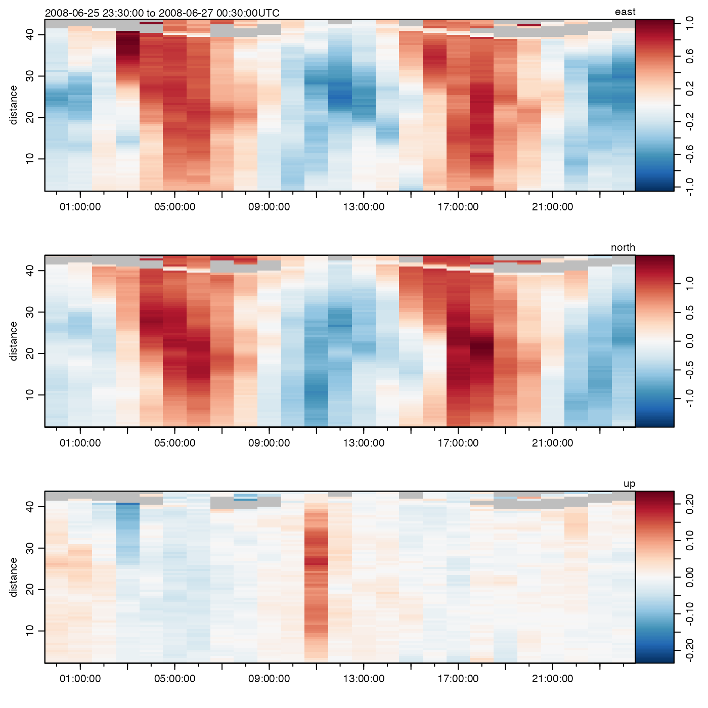
which=1:4 (or which="u1" to "u4") yield a distance-time image plot of a velocity component. If x is in beam coordinates (signalled by metadata$oce.coordinate=="beam"), this will be the beam velocity, labelled b[1] etc. If x is in xyz coordinates (sometimes called frame coordinates, or ship coordinates), it will be the velocity component to the right of the frame or ship (labelled u etc). Finally, if x is in "enu" coordinates, the image will show the the eastward component (labelled east). If x is in "other" coordinates, it will be component corresponding to east, after rotation (labelled u\'). Note that the coordinate is set by read.adp(), or by beamToXyzAdp(), xyzToEnuAdp(), or enuToOtherAdp().
which=5:8 (or which="a1" to "a4") yield distance-time images of backscatter intensity of the respective beams. (For data derived from Teledyne-RDI instruments, this is the item called ``echo intensity.'')
which=9:12 (or which="q1" to "q4") yield distance-time images of signal quality for the respective beams. (For RDI data derived from instruments, this is the item called ``correlation magnitude.'')
which=60 or which="map" draw a map of location(s).
which=70:73 (or which="g1" to "g4") yield distance-time images of percent-good for the respective beams. (For data derived from Teledyne-RDI instruments, which are the only instruments that yield this item, it is called ``percent good.'')
which=80:83 (or which="vv", which="va", which="vq", and which="vg") yield distance-time images of the vertical beam fields for a 5 beam "SentinelV" ADCP from Teledyne RDI.
which="vertical" yields a two panel distance-time image of vertical beam velocity and amplitude.
which=13 (or which="salinity") yields a time-series plot of salinity.
which=14 (or which="temperature") yields a time-series plot of temperature.
which=15 (or which="pressure") yields a time-series plot of pressure.
which=16 (or which="heading") yields a time-series plot of instrument heading.
which=17 (or which="pitch") yields a time-series plot of instrument pitch.
which=18 (or which="roll") yields a time-series plot of instrument roll.
which=19 yields a time-series plot of distance-averaged velocity for beam 1, rightward velocity, eastward velocity, or rotated-eastward velocity, depending on the coordinate system.
which=20 yields a time-series of distance-averaged velocity for beam 2, foreward velocity, northward velocity, or rotated-northward velocity, depending on the coordinate system.
which=21 yields a time-series of distance-averaged velocity for beam 3, up-frame velocity, upward velocity, or rotated-upward velocity, depending on the coordinate system.
which=22 yields a time-series of distance-averaged velocity for beam 4, for beam coordinates, or velocity estimate, for other coordinates. (This is ignored for 3-beam data.)
which="progressiveVector" (or which=23) yields a progressive-vector diagram in the horizontal plane, plotted with asp=1. Normally, the depth-averaged velocity components are used, but if the control list contains an item named bin, then the depth bin will be used (with an error resulting if the bin is out of range).
which=24 yields a time-averaged profile of the first component of velocity (see which=19 for the meaning of the component, in various coordinate systems).
which=25 as for 24, but the second component.
which=26 as for 24, but the third component.
which=27 as for 24, but the fourth component (if that makes sense, for the given instrument).
which=28 or "uv" yields velocity plot in the horizontal plane, i.e. u[2] versus u[1]. If the number of data points is small, a scattergraph is used, but if it is large, smoothScatter() is used.
which=29 or "uv+ellipse" as the "uv" case, but with an added indication of the tidal ellipse, calculated from the eigen vectors of the covariance matrix.
which=30 or "uv+ellipse+arrow" as the "uv+ellipse" case, but with an added arrow indicating the mean current.
which=40 or "bottomRange" for average bottom range from all beams of the instrument.
which=41 to 44 (or "bottomRange1" to "bottomRange4") for bottom range from beams 1 to 4.
which=50 or "bottomVelocity" for average bottom velocity from all beams of the instrument.
which=51 to 54 (or "bottomVelocity1" to "bottomVelocity4") for bottom velocity from beams 1 to 4.
which=55 (or "heaving") for time-integrated, depth-averaged, vertical velocity, i.e. a time series of heaving.
which=60 (or "map") for a map.
which=100 (or "soundSpeed") for a time series of sound speed.
which=200 (or "accelerometerx") for a time-series of the x component of the accelerometer reading.
which=201 (or "accelerometery") for a time-series of the y component of the accelerometer reading.
which=202 (or "accelerometerz") for a time-series of the z component of the accelerometer reading.
which=210 (or "magnetometerx") for a time-series of the x component of the magnetometer reading.
which=211 (or "magnetometery") for a time-series of the y component of the magnetometer reading.
which=212 (or "magnetometerz") for a time-series of the z component of the magnetometer reading.

In addition to the above, the following shortcuts are defined:

which="velocity" equivalent to which=1:3 or 1:4 (depending on the device) for velocity components.
which="amplitude" equivalent to which=5:7 or 5:8 (depending on the device) for backscatter intensity components.
which="quality" equivalent to which=9:11 or 9:12 (depending on the device) for quality components.
which="hydrography" equivalent to which=14:15 for temperature and pressure.
which="angles" equivalent to which=16:18 for heading, pitch and roll.
which="accelerometer" to plot a 3-panel timeseries of acceleration, equivalent to which=110:102.

The color scheme for image plots (which in 1:12) is provided by the col argument, which is passed to image() to do the actual plotting. See “Examples” for some comparisons.

A common quick-look plot to assess mooring movement is to use which=15:18 (pressure being included to signal the tide, and tidal currents may dislodge a mooring or cause it to settle).

By default, plot,adp-method uses a zlim value for the image() that is constructed to contain all the data, but to be symmetric about zero. This is done on a per-panel basis, and the scale is plotted at the top-right corner, along with the name of the variable being plotted. You may also supply zlim as one of the ... arguments, but be aware that a reasonable limit on horizontal velocity components is unlikely to be of much use for the vertical component.

A good first step in the analysis of measurements made from a moored device (stored in d, say) is to do plot(d, which=14:18). This shows time series of water properties and sensor orientation, which is helpful in deciding which data to trim at the start and end of the deployment, because they were measured on the dock or on the ship as it travelled to the mooring site.

Author

Dan Kelley

Examples

library(oce)
data(adp)
plot(adp, which = 1:3)

plot(adp, which = "temperature", tformat = "%H:%M")

Arguments

Value

Details

See also

Author

Examples