Plot a sealevel Object

Creates a plot for a sea-level dataset, in one of two varieties. Depending on the length of which, either a single-panel or multi-panel plot is drawn. If there is just one panel, then the value of par used in plot,sealevel-method is retained upon exit, making it convenient to add to the plot. For multi-panel plots, par is returned to the value it had before the call.

# S4 method for sealevel
plot(
  x,
  which = 1:3,
  drawTimeRange = getOption("oceDrawTimeRange"),
  mgp = getOption("oceMgp"),
  mar = c(mgp[1] + 0.5, mgp[1] + 1.5, mgp[2] + 1, mgp[2] + 3/4),
  marginsAsImage = FALSE,
  grid = TRUE,
  xlim,
  ylim,
  xaxs = "i",
  yaxs = "r",
  debug = getOption("oceDebug"),
  ...
)

Arguments

x: a sealevel object.
which: a numerical or string vector indicating desired plot types, with possibilities 1 or "all" for a time-series of all the elevations, 2 or "month" for a time-series of just the first month, 3 or "spectrum" for a power spectrum (truncated to frequencies below 0.1 cycles per hour, or 4 or "cumulativespectrum" for a cumulative integral of the power spectrum.
drawTimeRange: boolean that applies to panels with time as the horizontal axis, indicating whether to draw the time range in the top-left margin of the plot.
mgp: 3-element numerical vector to use for par("mgp"), and also for par("mar"), computed from this. The default is tighter than the R default, in order to use more space for the data and less for the axes.
mar: value to be used with par("mar").
marginsAsImage: logical value indicating whether to put a wide margin to the right of time-series plots, matching the space used up by a palette in an imagep() plot.
grid: logical value, indicating whether to draw a grid with grid().
xlim, ylim: optional limits for axes. If not supplied, reasonable choices will be made
xaxs, yaxs: axis-limit parameters, as for standard graphics. The default is to make the time axis extend to the edges of the box, but to make the y axis have some space above and below the range of the data.
debug: a flag that turns on debugging, if it exceeds 0.
...: optional arguments passed to plotting functions.

Value

None.

Historical Note

Until 2020-02-06, sea-level plots had the mean value removed, and indicated with a tick mark and margin note on the right-hand side of the plot. This behaviour was confusing. The change did not go through the usual deprecation process, because the margin-note behaviour had not been documented.

References

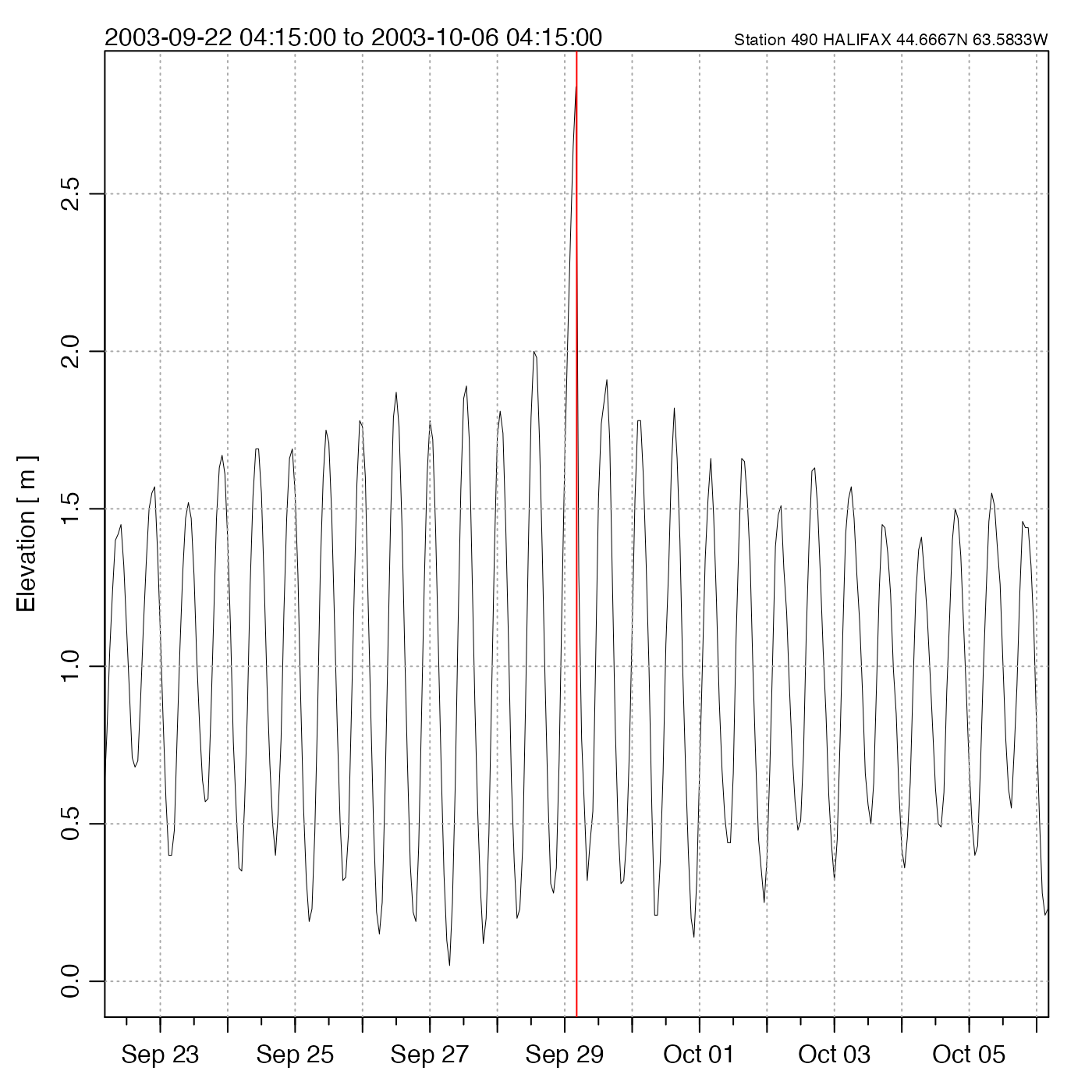
The example refers to Hurricane Juan, which caused a great deal of damage to Halifax in 2003. Since this was in the era of the digital photo, a casual web search will uncover some spectacular images of damage, from both wind and storm surge. Landfall, within 30km of this sealevel gauge, was between 00:10 and 00:20 Halifax local time on Monday, Sept 29, 2003.

Other functions that plot oce data: download.amsr(), plot,adp-method, plot,adv-method, plot,amsr-method, plot,argo-method, plot,bremen-method, plot,cm-method, plot,coastline-method, plot,ctd-method, plot,gps-method, plot,ladp-method, plot,landsat-method, plot,lisst-method, plot,lobo-method, plot,met-method, plot,odf-method, plot,rsk-method, plot,satellite-method, plot,section-method, plot,tidem-method, plot,topo-method, plot,windrose-method, plot,xbt-method, plotProfile(), plotScan(), plotTS(), tidem-class

Other things related to sealevel data: [[,sealevel-method, [[<-,sealevel-method, as.sealevel(), read.sealevel(), sealevel, sealevel-class, sealevelTuktoyaktuk, subset,sealevel-method, summary,sealevel-method

Author

Dan Kelley

Examples

library(oce)
data(sealevel)
# local Halifax time is UTC + 4h
juan <- as.POSIXct("2003-09-29 00:15:00", tz = "UTC") + 4 * 3600
plot(sealevel, which = 1, xlim = juan + 86400 * c(-7, 7))
abline(v = juan, col = "red")