6. Subclassing oce objects
Dan Kelley (https://orcid.org/0000-0001-7808-5911)
2026-04-19
Source:vignettes/F_subclassing.Rmd
F_subclassing.RmdAbstract. This vignette explains how to create new
object classes, using the low-level oce class as a
foundation. This scheme is beneficial, because the newly-formed objects
automatically gain the key properties of oce objects, in terms of
operators such as [[ and [[<-, functions
such as subset() and summary(), schemes for
handling units, etc. The setMethod() function is central to
the process of creating new classes, as will be illustrated here in a
practical way, using drifting-buoy data for example.
A drifting buoy
Data from buoy number 4201703 were downloaded from
http://www.coriolis.eu.org/Data-Products/Data-selection on
2022-01-09, by deselecting all data types except for “Drifting buoy”,
selecting a data window south of Nova Scotia and of area similar to that
province, expanding the tarball created by the website and then
focussing on the downloaded file named
"drifting-buoys-4201703.csv“.
There are many data in the source data file, but only a subset is
used here: starting with 300 samples of just five of the data fields:
time (called t for brevity), longitude (lon),
latitude (lat), temperature (Tatm) and
atmospheric pressure (Patm). This set was further trimmed
by removing data ensembles in which temperature was not reported. The
result was 146 observations of 5 variables. (Note that they are
not spaced uniformly in time, a feature that is of importance
only at the end of this document.)
The data were combined into a data frame named db and
packaged in an RDA file, an overview of which is provided as
follows.
library(oce)
#> Loading required package: gsw
load(system.file("extdata", "drifter.rda", package = "oce"))
str(db)
#> 'data.frame':    146 obs. of  5 variables:
#>  $ t   : POSIXct, format: "2021-11-01 21:04:00" "2021-11-01 23:04:00" ...
#>  $ lon : num  -62.7 -62.8 -62.8 -62.8 -62.8 ...
#>  $ lat : num  42.5 42.5 42.5 42.6 42.6 ...
#>  $ Tatm: num  19.2 19.2 19.2 19.2 19.2 ...
#>  $ Patm: num  1013 1014 1015 1016 1017 ...
Before showing how to create a new subclass, it will first be shown that such data could also be stored in the foundational class of the package.
Using the base oce class
The base class is named "oce", and so a new object of
that type can be created with
o <- new("oce")At this point, the summary() method does not reveal
much:
summary(o)
#> * Processing Log
#>
#>     - 2026-04-19 17:04:46 UTC: `Create oce object`
but if we populate the object with some data and metadata
o <- oceSetData(o, "time", db$t)
o <- oceSetData(o, "longitude", db$lon)
o <- oceSetData(o, "latitude", db$lat)
o <- oceSetMetadata(o, "ID", 4201703)
then the summary is more informative
summary(o)
#> * Time: 2021-11-01 21:04:00 to 2021-11-08 06:00:00 (146 samples, mean increment 1.054713 hour)
#> * Data Overview
#>
#>               Min.       Mean       Max.       Dim. NAs OriginalName
#>     time      1635800640 1636074398 1636351200 146  0   "-"
#>     longitude -63.011    -62.775    -62.636    146  0   "-"
#>     latitude  41.932     42.305     42.572     146  0   "-"
#>
#> * Processing Log
#>
#>     - 2026-04-19 17:04:46 UTC: `Create oce object`
#>     - 2026-04-19 17:04:46 UTC: `oceSetData(object = o, name = "time", value = db$t)`
#>     - 2026-04-19 17:04:46 UTC: `oceSetData(object = o, name = "longitude", value = db$lon)`
#>     - 2026-04-19 17:04:46 UTC: `oceSetData(object = o, name = "latitude", value = db$lat)`
#>     - 2026-04-19 17:04:46 UTC: `oceSetMetadata(object = o, name = "ID", value = 4201703)`
Note, however, that the ID is not listed by
summary(). This is because the general form of that
function is set up to focus on the contents of the data
slot, not the metadata slot. (Extending
summary() will described later.)
Objects of oce-class automatically have other methods,
besides summary(). For example, the accessing operator
[[ works for the object that was just created:
str(o[["latitude"]])
#>  num [1:146] 42.5 42.5 42.5 42.6 42.6 ...
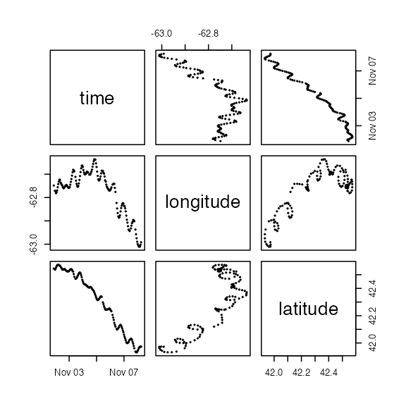
We can also use the default plot() function to show the
interdependence of entries in the data slot.
plot(o, pch = 20, cex = 0.5)
Figure 1. Demonstration of base-level plot().
Although this plot provides a useful overview of the data, it is not
something an analyst would consider publishing. To get more useful plot
types, we must create a new subclass that has a specialized
plot() method.
Creating a new subclass
A reasonable name for our new subclass might be
"drifter". With this choice, the class can be defined in a
single line of code:
drifter <- setClass(Class = "drifter", contains = "oce")Once this has been executed, the user can create a new object of this subclass with
d <- new("drifter")Although it is simple to add data and metadata as in the previous
section, it is more convenient to supply this information when
new() is used. To accomplish this, we must set up an
initialization function, as follows.
setMethod(
    f = "initialize",
    signature = "drifter",
    definition = function(.Object, time, longitude, latitude, ID = "unknown") {
        if (missing(time)) {
            stop("In new(drifter) : must provide 'time'", call. = FALSE)
        }
        if (missing(longitude)) {
            stop("In new(drifter) : must provide 'longitude'", call. = FALSE)
        }
        if (missing(latitude)) {
            stop("In new(drifter) : must provide 'latitude'", call. = FALSE)
        }
        .Object@data$time <- time
        .Object@data$longitude <- longitude
        .Object@data$latitude <- latitude
        .Object@metadata$ID <- ID
        .Object@processingLog$time <- presentTime()
        .Object@processingLog$value <- "create 'drifter' object"
        return(.Object)
    }
)
This method takes away the choice of where to put things (in
data or in metadata), saving users from having
to make that decision, possibly breaking other code. Also, note that
some error checking has been used here, so that an attempt to use
new("drifter") without providing time, etc., produces an
error message, as shown below.
d <- new("drifter")
Error: In new(drifter) : must provide 'time'
With this setup, we may now create an object that we can use for the rest of this vignette:
d <- new("drifter", time = db$t, longitude = db$lon, latitude = db$lat, ID = 4201703)and this will be used in the next three subsections, showing how to
specialize the plot() method, the summary()
method, and the [[ accessor. Note the use of
setMethod() in each instance.
Specializing the plot() function
The f, signature and
definition arguments follow the same pattern as in the
previous example, and readers ought to focus on last of these. Here,
three plot types are provided, as selected by an argument called
which. The first two give time-series plots of drifter
longitude and latitude, and the third shows the trajectory.
setMethod(
    f = "plot",
    signature = signature("drifter"),
    definition = function(x, which = 1, ...) {
        lonlab <- expression("Longitude [" * degree * "E]")
        latlab <- expression("Latitude [" * degree * "N]")
        if (which == 1) {
            oce.plot.ts(x[["time"]], x[["longitude"]],
                ylab = lonlab, ...
            )
        } else if (which == 2) {
            oce.plot.ts(x[["time"]], x[["latitude"]],
                ylab = latlab, ...
            )
        } else if (which == 3) {
            asp <- 1 / cos(mean(range(x[["latitude"]]) * pi / 180))
            plot(x[["longitude"]], x[["latitude"]],
                asp = asp, xlab = lonlab, ylab = latlab, ...
            )
        } else {
            stop("In plot,drifter-method : try which=1, 2 or 3", call. = FALSE)
        }
    }
)
The three plot types are fairly rudimentary, but the ...
argument can be used for customization, as in the following example.
par(mar = c(3.3, 3.3, 1, 1), mgp = c(2, 0.7, 0))
layout(matrix(c(1, 3, 2, 3), nrow = 2, byrow = TRUE))
plot(d, which = 1, drawTimeRange = FALSE)
plot(d, which = 2, drawTimeRange = FALSE)
plot(d, which = 3)
Figure 2. Demonstration of specialized plot().
Specializing the summary() function
Here, our sole purpose is to add an indication of the ID of the
drifter. The rest of the information provided by the base-level
summary() function will suffice to summarize the rest.
So, with
setMethod(
    f = "summary",
    signature = "drifter",
    definition = function(object, ...) {
        cat("CTD Summary\n-----------\n\n")
        cat("* ID:          ", object[["ID"]], "\n", sep = "")
        invisible(callNextMethod())
    }
)
An example follows.
summary(d)
#> CTD Summary
#> -----------
#>
#> * ID:          4201703
#> * Time: 2021-11-01 21:04:00 to 2021-11-08 06:00:00 (146 samples, mean increment 1.054713 hour)
#> * Data Overview
#>
#>               Min.       Mean       Max.       Dim. NAs
#>     time      1635800640 1636074398 1636351200 146  0
#>     longitude -63.011    -62.775    -62.636    146  0
#>     latitude  41.932     42.305     42.572     146  0
#>
#> * Processing Log
#>
#>     - 2026-04-19 17:04:47 UTC: `create 'drifter' object`
Specializing the [[ accessor
The variation of drifter position provides information on ocean
velocity, and this is of sufficient interest that it might be worth
adding to [[. This may be done as follows.
setMethod(
    f = "[[",
    signature(x = "drifter", i = "ANY", j = "ANY"),
    definition = function(x, i, j, ...) {
        if (i == "velocity") {
            D <- function(x) {
                dx <- diff(x)
                c(dx[1], dx)
            }
            lat <- x[["latitude"]]
            lon <- x[["longitude"]]
            dt <- D(as.numeric(x[["time"]])) # seconds
            scalex <- 111.12e3 # m per degree latitude
            scaley <- scalex * cos(lat * pi / 180)
            u <- scalex * D(lon) / dt
            v <- scaley * D(lat) / dt
            list(u = u, v = v)
        } else {
            callNextMethod()
        }
    }
)
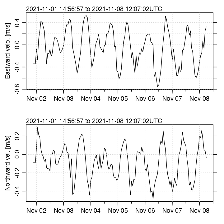
As a test, we can plot the velocity components.
uv <- d[["velocity"]]
par(mfrow = c(2, 1))
oce.plot.ts(d[["time"]], uv$u, ylab = "Eastward velo. [m/s]", grid = TRUE)
oce.plot.ts(d[["time"]], uv$v, ylab = "Northward vel. [m/s]", grid = TRUE)
Figure 3. Velocities inferred from drifter motion.
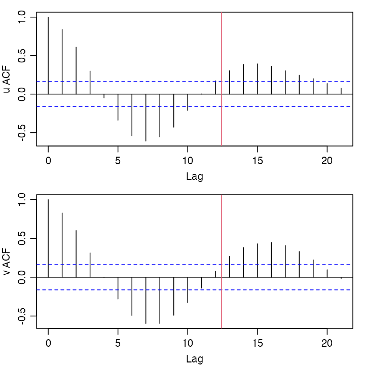
The acf() function, which computes lagged
autocorrelation, can shed some light on the periodicity of the velocity
signals (but see Exercise 3), as follows.
data(tidedata)
M2period <- 1 / with(tidedata$const, freq[[which(name == "M2")]])
uv <- d[["velocity"]]
par(mfrow = c(2, 1), mar = c(3, 3, 1, 1), mgp = c(2, 0.7, 0))
acf(uv$u, main = "", ylab = "u ACF")
abline(v = M2period, col = 2)
acf(uv$v, main = "", ylab = "v ACF")
abline(v = M2period, col = 2)
Figure 4. Autocorrelation analysis of drifter velocities, showing also the M2 period.
Summary
As has been illustrated above, the setMethod() function
is the key to altering generic functions such as plot(),
summary() and [[. The details of how this
works are explained in numerous manuals, books, and websites, but
impatient readers can save some time by simply copying and expanding on
the code provided in the previous sections.
Appendix: exercises for the reader
Add atmospheric temperature and pressure (both contained in the source RDA file) to the
drifterobject initialization function. Be sure to check that they were provided or, if you choose, let them be optional.Think of other useful plot types, and add these to the
plot()method.For the final lagged-autocorrelation function, use
approx()to get new time-series with a constant sampling rate.Again for the lagged-autocorrelation function, add a line for local Coriolis period.
As an alternative to the lagged-autocorrelation method, test for periodicity of velocity by using
nls(), supplied with a sinusoidal function that has adjustable amplitude, phase, and frequency.