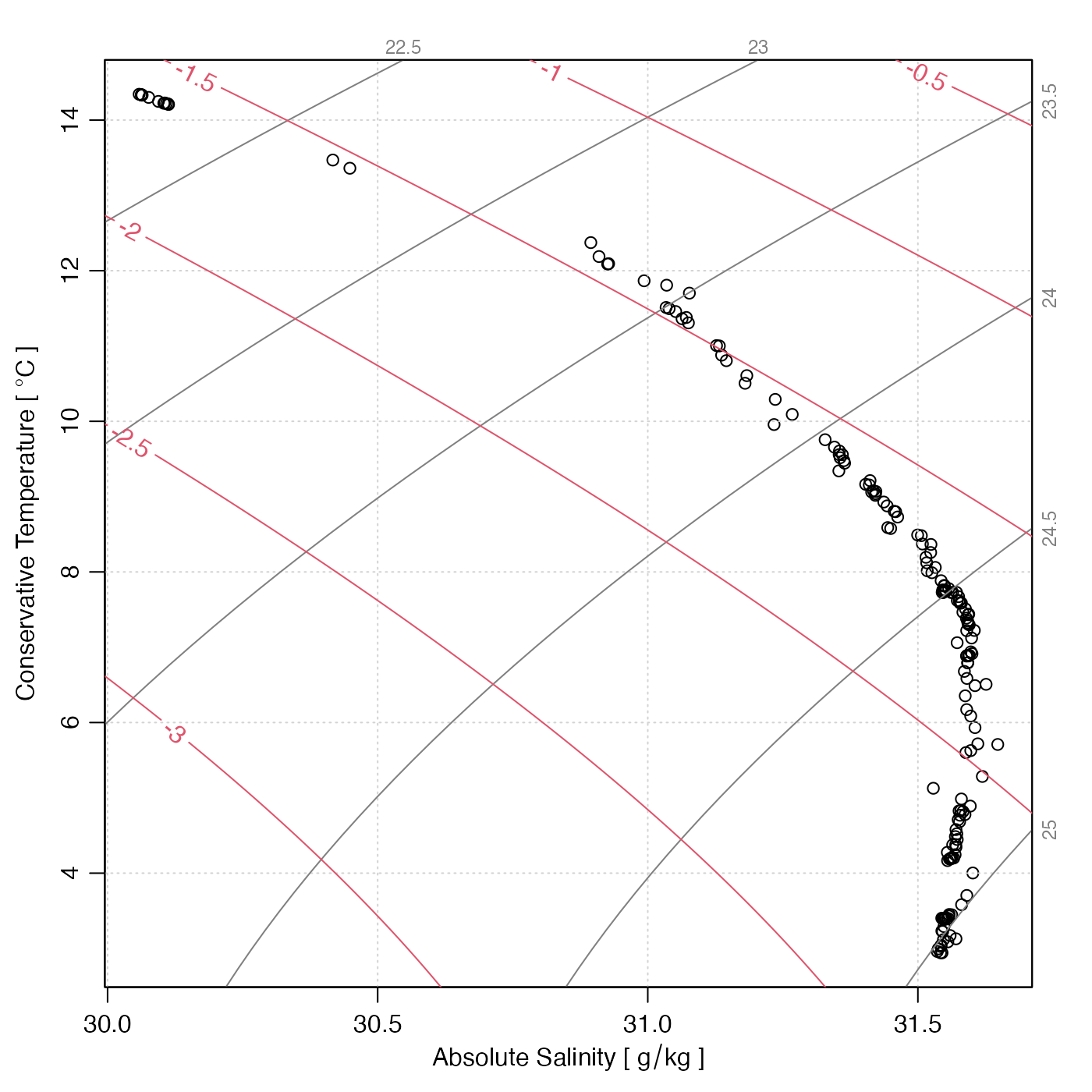
Plot Temperature-Salinity Diagram

Creates a temperature-salinity plot for a CTD cast, with labeled isopycnals.

Usage

plotTS(
  x,
  inSitu = FALSE,
  type = "p",
  referencePressure = 0,
  nlevels = 6,
  levels,
  grid = TRUE,
  col.grid = "lightgray",
  lty.grid = "dotted",
  rho1000 = FALSE,
  eos = getOption("oceEOS", default = "gsw"),
  cex = par("cex"),
  col = par("col"),
  pch = par("pch"),
  bg = "white",
  pt.bg = "transparent",
  col.rho = gray(0.5),
  cex.rho = 3/4 * par("cex"),
  rotate = TRUE,
  useSmoothScatter = FALSE,
  xlab,
  ylab,
  Slim,
  Tlim,
  drawFreezing = TRUE,
  trimIsopycnals = TRUE,
  gridIsopycnals = c(30, 50),
  mgp = getOption("oceMgp"),
  mar = c(mgp[1] + 1.5, mgp[1] + 1.5, mgp[1], mgp[1]),
  lwd = par("lwd"),
  lty = par("lty"),
  lwd.rho = par("lwd"),
  lty.rho = par("lty"),
  add = FALSE,
  inset = FALSE,
  debug = getOption("oceDebug"),
  ...
)

Arguments

x: a ctd, argo or section object, or a list containing solely ctd objects or argo objects.
inSitu: A boolean indicating whether to use in-situ temperature or (the default) potential temperature, calculated with reference pressure given by referencePressure. This is ignored if eos="gsw", because those cases the y axis is necessarily the conservative formulation of temperature.
type: representation of data, "p" for points, "l" for connecting lines, "b" for spaced connecting lines, or "n" for no indication.
referencePressure: reference pressure, to be used in calculating potential temperature, if inSitu is FALSE.
nlevels: Number of automatically-selected isopycnal levels (ignored if levels is supplied).
levels: Optional vector of desired isopycnal levels.
grid: a flag that can be set to TRUE to get a grid.
col.grid: color for grid.
lty.grid: line type for grid.
rho1000: if TRUE, label isopycnals as e.g. 1024; if FALSE, label as e.g. 24
eos: equation of state to be used, either "unesco" or "gsw".
cex: character-expansion factor for symbols, as in par("cex").
col: color for symbols.
pch: symbol type, as in par("pch").
bg: optional color to be painted under plotting area, before plotting. (This is useful for cases in which inset=TRUE.)
pt.bg: inside color for symbols with pch in 21:25
col.rho: color for isopycnal lines and their labels.
cex.rho: size of the isopycnal labels.
rotate: if TRUE, labels in right-hand margin are written vertically
useSmoothScatter: if TRUE, use smoothScatter() to plot the points.
xlab: optional label for the x axis, with default "Salinity [PSU]".
ylab: optional label for the y axis, with default "Temperature [C]".
Slim: optional limits for salinity axis, otherwise inferred from visible data (i.e. the data that have finite values for both salinity and temperature).
Tlim: as Slim, but for temperature.
drawFreezing: logical indication of whether to draw a freezing-point line. This is based on zero pressure. If eos="unesco" then swTFreeze() is used to compute the curve, whereas if eos="gsw" then gsw::gsw_CT_freezing() is used; in each case, zero pressure is used.
trimIsopycnals: logical value (TRUE by default) that indicates whether to trim isopycnal curves to the region of temperature-salinity space for which density computations are considered to be valid in the context of the chosen eos; see “Details”.
gridIsopycnals: a parameter that controls how the isopycnals are computed. This may be NULL, or an integer vector of length 2. Case 1: the isopycnals are drawn by tracing density isopleths in salinity-temperature space. This method was used as the default prior to version 1.7-11, but it was found to yield staircase-like isopycnal curves for highly zoomed-in plots (e.g. with millidegree temperature ranges). Case 2: a grid of density is constructed, with gridIsopycnals[1] salinity levels and gridIsopycnals[2] temperature levels, and then contourLines() is used to trace the isopycnals.
mgp: 3-element numerical vector to use for [par](mgp), and also for par(mar), computed from this. The default is tighter than the R default, in order to use more space for the data and less for the axes.
mar: value to be used with par("mar"). If set to NULL, then par("mar") is used. A good choice for a TS diagram with a palette to the right is mar=par("mar")+c(0, 0, 0, 1)).
lwd: line width of lines or symbols.
lty: line type of lines or symbols.
lwd.rho: line width for density curves.
lty.rho: line type for density curves.
add: a flag that controls whether to add to an existing plot. (It makes sense to use add=TRUE in the panel argument of a coplot(), for example.)
inset: set to TRUE for use within plotInset(). The effect is to prevent the present function from adjusting margins, which is necessary because margin adjustment is the basis for the method used by plotInset().
debug: a flag that turns on debugging. Set to 1 to get a moderate amount of debugging information, or to 2 to get more.
...: optional arguments passed to plotting functions.

Value

A list is silently returned, containing xat and yat, values that can be used by oce.grid() to add a grid to the plot.

Details

The isopycnal curves (along which density is constant) are drawn with drawIsopycnals(), which also places labels in the margins showing density minus 1000 \(kg/m^3\). If trimIsopycnals is TRUE (which is the default), these curves are trimmed to the region within which the results of density calculation in the chosen equation of state (eos) are considered to be reliable.

With eos="unesco" this region includes Practical Salinity from 0 to 42 and Potential Temperature from -2C to 40C, in accordance with Fofonoff and Millard (1983, page 23).

With eos="gsw" the lower limit of Absolute Salinity validity is taken as 0 g/kg, in accordance with both McDougall et al. (2003 section 3) and the TEOS-10/gsw Matlab code for the so-called "funnel" of validity. However, an appropriate upper limit on Absolute Salinity is not as clear. Here, the value 42 g/kg is chosen to match the "funnel" Matlab code as of July 2020, but two other choices might have been made. One is 50 g/kg, since gsw::gsw_SA_from_rho() returns NA values for Absolute Salinities exceeding that value, and another is 40 g/kg, as in McDougall et al. (2003 section 3). The Conservative Temperature range is set to run from -2C to 33C, as in McDougall et al. (2003 section 3), even though the "funnel" imposes no upper limit on this variable.

References

Fofonoff, N. P., and R. C. Millard. "Algorithms for Computation of Fundamental Properties of Seawater." UNESCO Technical Papers in Marine Research. SCOR working group on Evaluation of CTD data; UNESCO/ICES/SCOR/IAPSO Joint Panel on Oceanographic Tables and Standards, 1983. https://unesdoc.unesco.org/ark:/48223/pf0000059832.
McDougall, Trevor J., David R. Jackett, Daniel G. Wright, and Rainer Feistel. "Accurate and Computationally Efficient Algorithms for Potential Temperature and Density of Seawater." Journal of Atmospheric and Oceanic Technology 20, no. 5 (May 1, 2003): 730-41. https://journals.ametsoc.org/jtech/article/20/5/730/2543/Accurate-and-Computationally-Efficient-Algorithms.

Author

Dan Kelley

Examples

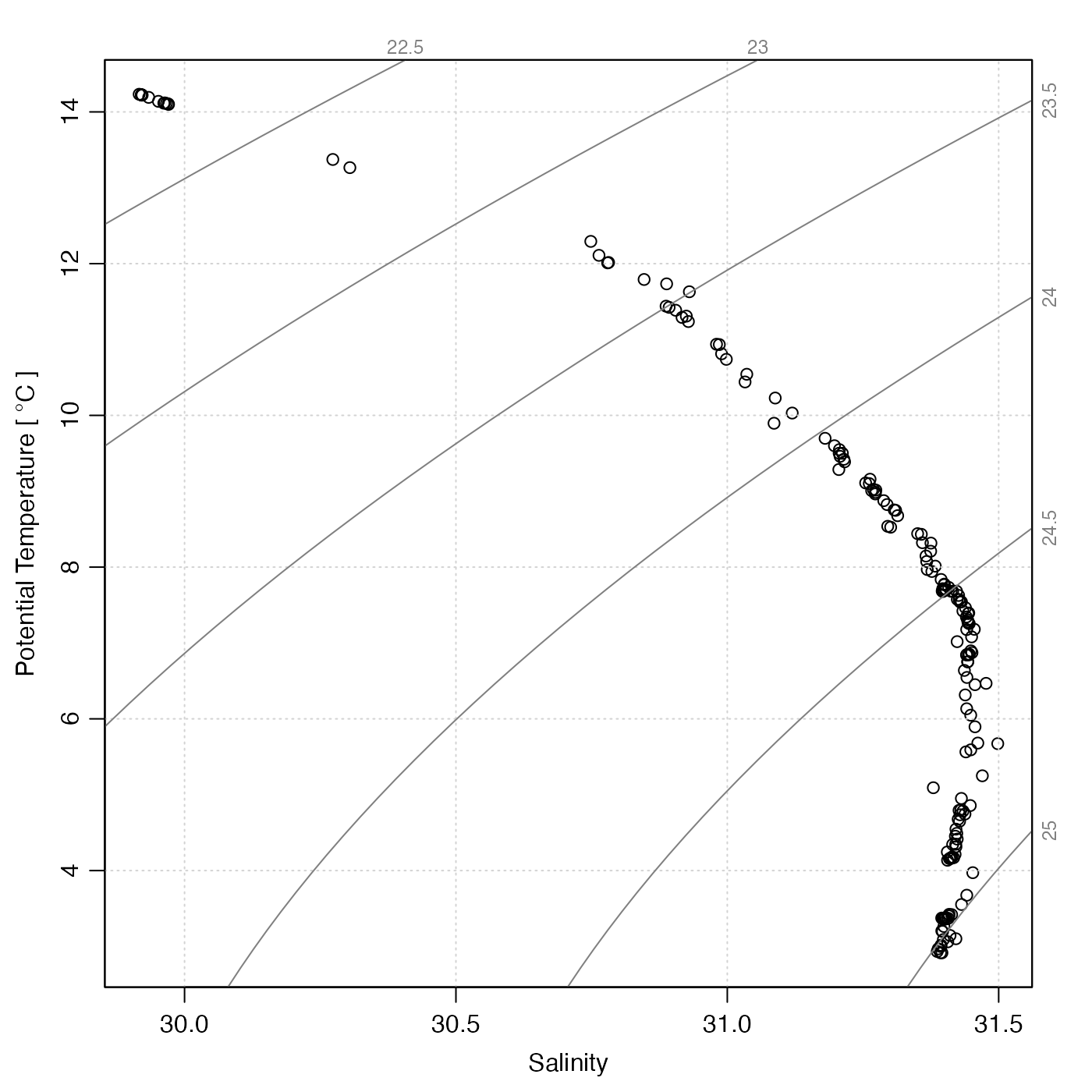
# 1. ctd object
library(oce)
data(ctd)
plotTS(ctd)


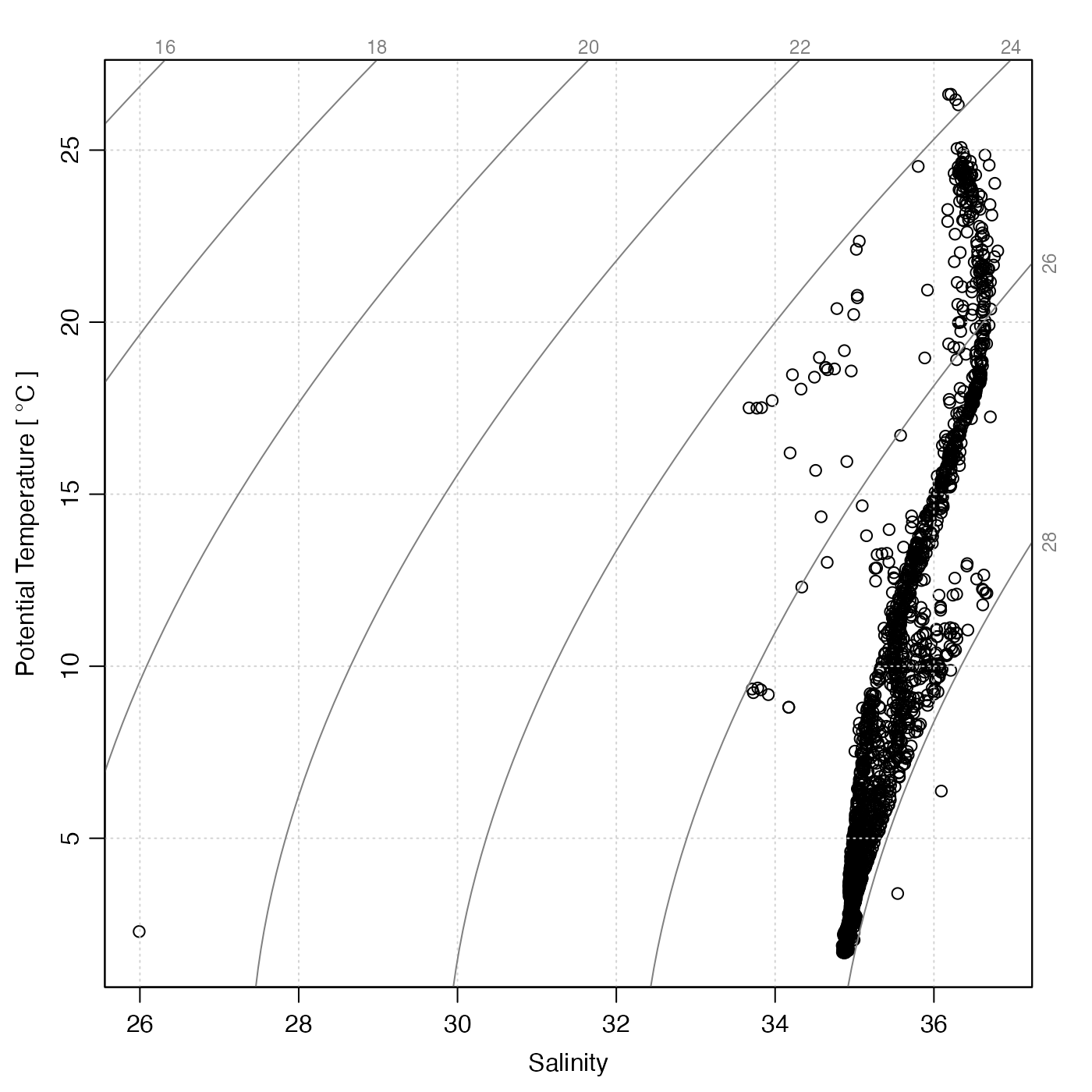
# 2. section object (note the outlier!)
data(section)
plotTS(section)


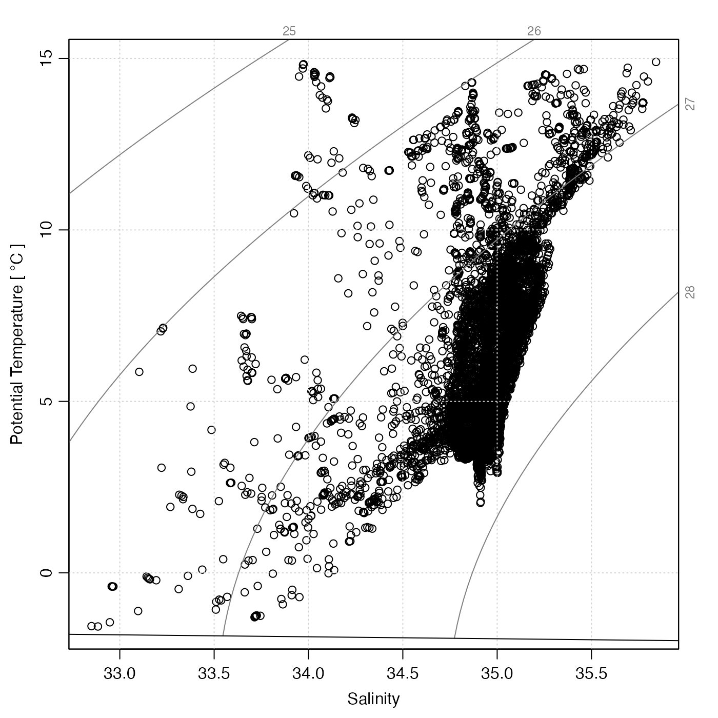
# 3. argo object
data(argo)
plotTS(handleFlags(argo))


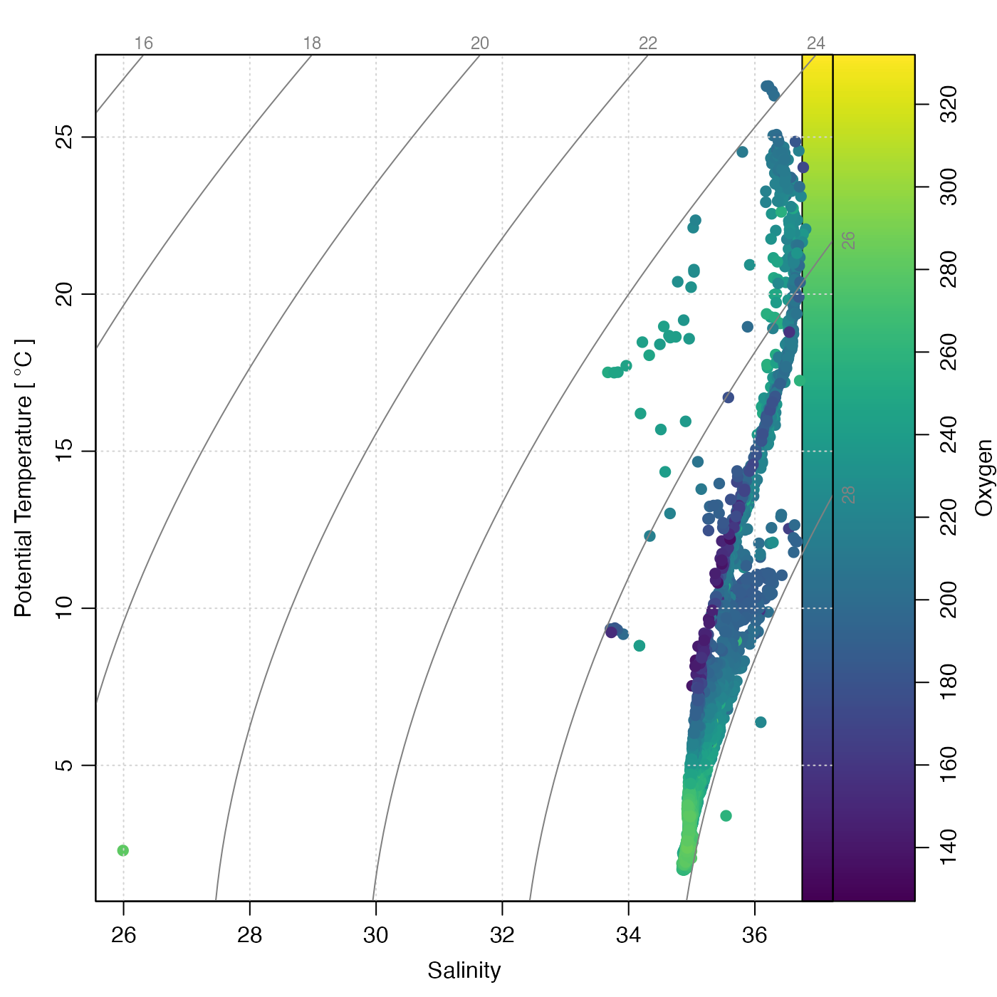
# 4. oxygen-based colormap
marOrig <- par("mar") # so later plots with palettes have same margins
cm <- colormap(section[["oxygen"]])
drawPalette(colormap = cm, zlab = "Oxygen")
plotTS(section, pch = 19, col = cm$zcol, mar = par("mar")) # the mar adjusts for the palette


# 5. waters near Gulf Stream, colour-coded for longitude.
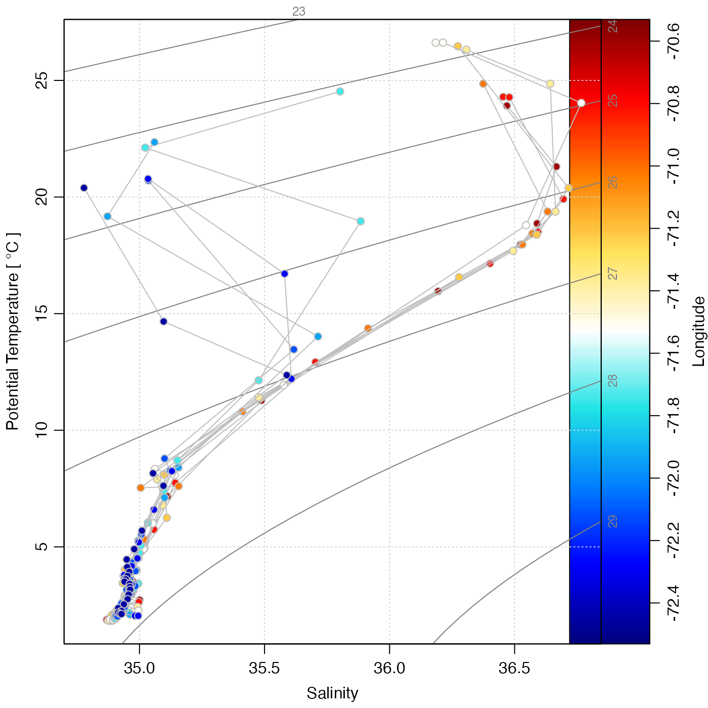
sec <- subset(section, abs(longitude + 71.6) < 1)
cm <- colormap(sec[["longitude", "byStation"]], col = oceColors9B)
par(mar = c(3.3, 3.3, 1, 1.5))
drawPalette(colormap = cm, zlab = "Longitude")
plotTS(sec, type = "n", xaxs = "r", mar = par("mar"))
jnk <- mapply(
    function(s, col) {
        plotTS(s, type = "o", col = "gray", pt.bg = col, pch = 21, add = TRUE)
    },
    sec[["station"]],
    col = cm$zcol
)


# 6. with added spiciness contours
data(ctd)
plotTS(ctd, eos = "gsw") # MANDATORY so x=SA and y=CT
usr <- par("usr")
n <- 100
SAgrid <- seq(usr[1], usr[2], length.out = n)
CTgrid <- seq(usr[3], usr[4], length.out = n)
g <- expand.grid(SA = SAgrid, CT = CTgrid)
spiciness <- matrix(gsw::gsw_spiciness0(g$SA, g$CT), nrow = n)
contour(SAgrid, CTgrid, spiciness, col = 2, labcex = 1, add = TRUE)