Plot a rsk Object

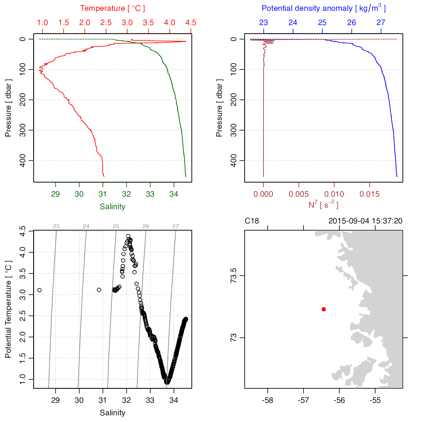
Rsk data may be in many forms, and it is not easy to devise a general plotting strategy for all of them. The present function is quite crude, on the assumption that users will understand their own datasets, and that they can devise plots that are best-suited to their applications. Sometimes, the sensible scheme is to coerce the object into another form, e.g. using plot(as.ctd(rsk)) if the object contains CTD-like data. Other times, users should extract data from the rsk object and construct plots themselves. The idea is to use the present function mainly to get an overview, and for that reason, the default plot type (set by which) is a set of time-series plots, because the one thing that is definitely known about rsk objects is that they contain a time vector in their data slot.

Usage

# S4 method for class 'rsk'
plot(
  x,
  which = "timeseries",
  tlim,
  ylim,
  xlab,
  ylab,
  tformat,
  drawTimeRange = getOption("oceDrawTimeRange"),
  abbreviateTimeRange = getOption("oceAbbreviateTimeRange"),
  useSmoothScatter = FALSE,
  mgp = getOption("oceMgp"),
  mar = c(mgp[1] + 1.5, mgp[1] + 1.5, 1.5, 1.5),
  main = "",
  debug = getOption("oceDebug"),
  ...
)

Arguments

x

an rsk object.

which

character indicating desired plot types. These are graphed in panels running down from the top of the page. See “Details” for the meanings of various values of which.

tlim

optional limits for time axis. If not provided, the value will be inferred from the data.

ylim

optional limits for the y axis. If not provided, the value will be inferred from the data. (It is helpful to specify this, if the auto-scaled value will be inappropriate, e.g. if more lines are to be added later). Note that this is ignored, unless length(which) == 1 and which corresponds to one of the data fields. If a multipanel plot of a specific subset of the data fields is desired with ylim control, it should be done panel by panel (see Examples).

xlab

optional label for x axis.

ylab

optional label for y axis.

tformat

optional argument passed to oce.plot.ts(), for plot types that call that function. (See strptime() for the format used.)

drawTimeRange

boolean that applies to panels with time as the horizontal axis, indicating whether to draw the time range in the top-left margin of the plot.

abbreviateTimeRange

boolean that applies to panels with time as the horizontal axis, indicating whether to abbreviate the second time in the time range (e.g. skipping the year, month, day, etc. if it's the same as the start time).

useSmoothScatter

a boolean to cause smoothScatter() to be used for profile plots, instead of plot().

mgp

3-element numerical vector to use for par("mgp"), and also for par(mar), computed from this. The default is tighter than the R default, in order to use more space for the data and less for the axes.

mar

value to be used with par("mar").

main

main title for plot, used just on the top panel, if there are several panels.

debug

a flag that turns on debugging, if it exceeds 0.

...

optional arguments passed to plotting functions.

Details

Plots produced are time series plots of the data in the object. The default, which="timeseries" plots all data fields, and over-rides any other specification. Specific fields can be plotted by naming the field, e.g. which="temperature" to plot a time series of just the temperature field.

See also

The documentation for rsk explains the structure of rsk objects, and also outlines the other functions dealing with them.

Other functions that plot oce data: download.amsr(), plot,adp-method, plot,adv-method, plot,amsr-method, plot,argo-method, plot,bremen-method, plot,cm-method, plot,coastline-method, plot,ctd-method, plot,gps-method, plot,ladp-method, plot,landsat-method, plot,lisst-method, plot,lobo-method, plot,met-method, plot,odf-method, plot,satellite-method, plot,sealevel-method, plot,section-method, plot,tidem-method, plot,topo-method, plot,windrose-method, plot,xbt-method, plotProfile(), plotScan(), plotTS(), tidem-class

Other things related to rsk data: [[,rsk-method, [[<-,rsk-method, as.rsk(), ctdFindProfilesRBR(), read.rsk(), rsk, rsk-class, rskPatm(), rskToc(), subset,rsk-method, summary,rsk-method

Author

Dan Kelley and Clark Richards

Examples

library(oce)
data(rsk)
# 1. default timeseries plot of all data fields
plot(rsk)

# 2. plot in ctd format
plot(as.ctd(rsk))