Plot a summary diagram for argo data.
Usage
# S4 method for class 'argo'
plot(
  x,
  which = 1,
  level,
  coastline = c("best", "coastlineWorld", "coastlineWorldMedium", "coastlineWorldFine",
    "none"),
  cex = 1,
  pch = 1,
  type = "p",
  col = 1,
  fill = FALSE,
  projection = NULL,
  mgp = getOption("oceMgp"),
  mar = c(mgp[1] + 1.5, mgp[1] + 1.5, 1.5, 1.5),
  tformat,
  debug = getOption("oceDebug"),
  ...
)
Arguments
- x
an argo object.
- which
list of desired plot types, one of the following. Note that
oce.pmatch()is used to try to complete partial character matches, and that an error will occur if the match is not complete (e.g."salinity"matches to both"salinity ts"and"salinity profile".).which=1,which="trajectory"orwhich="map"gives a plot of the argo trajectory, with the coastline, if one is provided.which=2or"salinity ts"gives a time series of salinity at the indicated level(s)which=3or"temperature ts"gives a time series of temperature at the indicated level(s)which=4or"TS"gives a TS diagram at the indicated level(s)which=5or"salinity profile"gives a salinity profilewhich=6or"temperature profile"gives a temperature profilewhich=7or"sigma0 profile"gives a sigma0 profilewhich=8or"spice profile"gives a spiciness profile, referenced to the surface. (This is the same as usingwhich=9.)which=9or"spiciness0 profile"gives a profile of spiciness referenced to a pressure of 0 dbar, i.e. the surface. (This is the same as usingwhich=8.)which=10or"spiciness1 profile"gives a profile of spiciness referenced to a pressure of 1000 dbar.which=11or"spiciness2 profile"gives a profile of spiciness referenced to a pressure of 2000 dbar.
- level
depth pseudo-level to plot, for
which=2and higher. May be an integer, in which case it refers to an index of depth (1 being the top) or it may be the string "all" which means to plot all data.- coastline
character string giving the coastline to be used in an Argo-location map, or
"best"to pick the one with highest resolution, or"none"to avoid drawing the coastline.- cex
size of plotting symbols to be used if
type="p".- pch
type of plotting symbols to be used if
type="p".- type
plot type, either
"l"or"p".- col
optional list of colors for plotting.
- fill
either a logical, indicating whether to fill the land with light-gray, or a color name. Owing to problems with some projections, the default is not to fill.
- projection
character value indicating the projection to be used in trajectory maps. If this is
NULL, no projection is used, although the plot aspect ratio will be set to yield zero shape distortion at the mean float latitude. Ifprojection="automatic", then one of two projections is used: stereopolar (i.e."+proj=stere +lon_0=X"whereXis the mean longitude), or Mercator (i.e."+proj=merc") otherwise. Otherwise,projectionmust be a character string specifying a projection in the notation used byoceProject()andmapPlot().- mgp
a 3-element numerical vector to use for
par(mgp), and also forpar(mar), computed from this. The default is tighter than the R default, in order to use more space for the data and less for the axes.- mar
value to be used with
par("mar").- tformat
optional argument passed to
oce.plot.ts(), for plot types that call that function. (Seestrptime()for the format used.)- debug
debugging flag.
- ...
optional arguments passed to plotting functions.
See also
Other things related to argo data:
D4902337_219.nc,
[[,argo-method,
[[<-,argo-method,
argo,
argo-class,
argo2ctd(),
argoGrid(),
argoNames2oceNames(),
as.argo(),
handleFlags,argo-method,
read.argo(),
read.argo.copernicus(),
subset,argo-method,
summary,argo-method
Other functions that plot oce data:
plot,adp-method,
plot,adv-method,
plot,amsr-method,
plot,bremen-method,
plot,cm-method,
plot,coastline-method,
plot,ctd-method,
plot,gps-method,
plot,ladp-method,
plot,landsat-method,
plot,lisst-method,
plot,lobo-method,
plot,met-method,
plot,odf-method,
plot,rsk-method,
plot,satellite-method,
plot,sealevel-method,
plot,section-method,
plot,tidem-method,
plot,topo-method,
plot,windrose-method,
plot,xbt-method,
plotProfile(),
plotScan(),
plotTS()
Examples
library(oce)
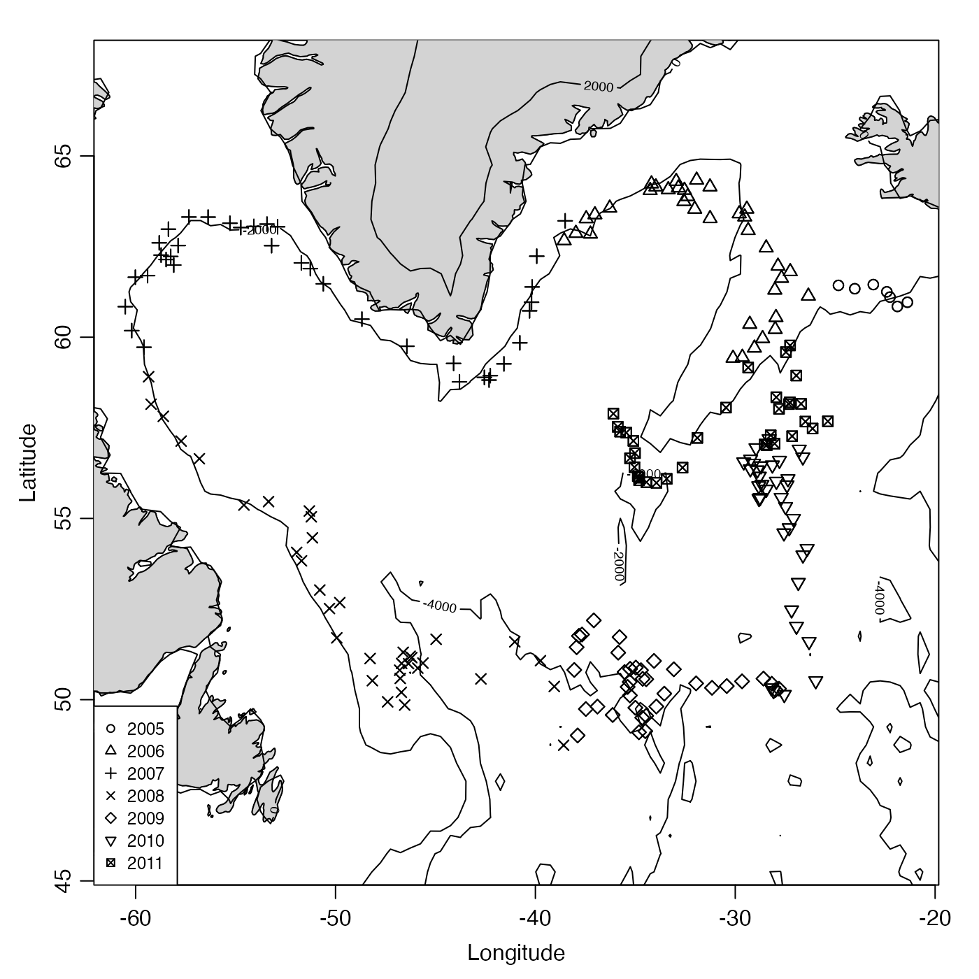
data(argo)
tc <- cut(argo[["time"]], "year")
# Example 1: plot map, which reveals float trajectory.
plot(argo, pch = as.integer(tc))
year <- substr(levels(tc), 1, 4)
data(topoWorld)
contour(topoWorld[["longitude"]], topoWorld[["latitude"]],
topoWorld[["z"]],
add = TRUE
)
legend("bottomleft", pch = seq_along(year), legend = year, bg = "white", cex = 3 / 4)
 # Example 2: plot map, TS, T(z) and S(z). Note the use
# of handleFlags(), to skip over questionable data.
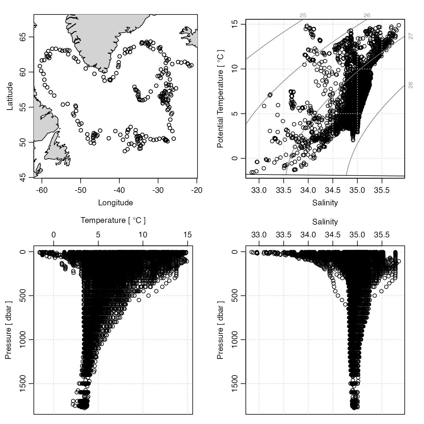
plot(handleFlags(argo), which = c(1, 4, 6, 5))
# Example 2: plot map, TS, T(z) and S(z). Note the use
# of handleFlags(), to skip over questionable data.
plot(handleFlags(argo), which = c(1, 4, 6, 5))