Class to Store Acoustic-Doppler Profiler Data

This class stores data from acoustic Doppler profilers. Some manufacturers call these ADCPs, while others call them ADPs; here the shorter form is used by analogy to ADVs.

Slots

data: As with all oce objects, the data slot for adp objects is a list containing the main data for the object. The key items stored in this slot include time, distance, and v, along with angles heading, pitch and roll.
metadata: As with all oce objects, the metadata slot for adp objects is a list containing information about the data or about the object itself. Examples that are of common interest include oceCoordinate, orientation, frequency, and beamAngle.
processingLog: As with all oce objects, the processingLog slot for adp objects is a list with entries describing the creation and evolution of the object. The contents are updated by various oce functions to keep a record of processing steps. Object summaries and processingLogShow() both display the log.

Modifying slot contents

Although the [[<- operator may permit modification of the contents of adp objects (see [[<-,adp-method), it is better to use oceSetData() and oceSetMetadata(), because those functions save an entry in the processingLog that describes the change.

Retrieving slot contents

The full contents of the data and metadata slots of a adp object may be retrieved in the standard R way using slot(). For example slot(o,"data") returns the data slot of an object named o, and similarly slot(o,"metadata") returns the metadata slot.

The slots may also be obtained with the [[,adp-method operator, as e.g. o[["data"]] and o[["metadata"]], respectively.

The [[,adp-method operator can also be used to retrieve items from within the data and metadata slots. For example, o[["temperature"]] can be used to retrieve temperature from an object containing that quantity. The rule is that a named quantity is sought first within the object's metadata slot, with the data slot being checked only if metadata does not contain the item. This [[ method can also be used to get certain derived quantities, if the object contains sufficient information to calculate them. For example, an object that holds (practical) salinity, temperature and pressure, along with longitude and latitude, has sufficient information to compute Absolute Salinity, and so o[["SA"]] will yield the calculated Absolute Salinity.

It is also possible to find items more directly, using oceGetData() and oceGetMetadata(), but neither of these functions can retrieve derived items.

Reading/creating `adp` objects

The metadata slot contains various items relating to the dataset, including source file name, sampling rate, velocity resolution, velocity maximum value, and so on. Some of these are particular to particular instrument types, and prudent researchers will take a moment to examine the whole contents of the metadata, either in summary form (with str(adp[["metadata"]])) or in detail (with adp[["metadata"]]). Perhaps the most useful general properties are adp[["bin1Distance"]] (the distance, in metres, from the sensor to the bottom of the first bin), adp[["cellSize"]] (the cell height, in metres, in the vertical direction, not along the beam), and adp[["beamAngle"]] (the angle, in degrees, between beams and an imaginary centre line that bisects all beam pairs).

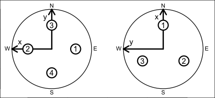
The diagram provided below indicates the coordinate-axis and beam-numbering conventions for three- and four-beam ADP devices, viewed as though the reader were looking towards the beams being emitted from the transducers.

Figure: adp_beams.png

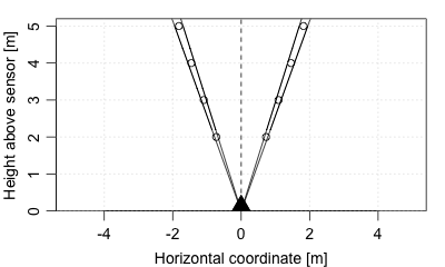
The bin geometry of a four-beam profiler is illustrated below, for adp[["beamAngle"]] equal to 20 degrees, adp[["bin1Distance"]] equal to 2m, and adp[["cellSize"]] equal to 1m. In the diagram, the viewer is in the plane containing two beams that are not shown, so the two visible beams are separated by 40 degrees. Circles indicate the centres of the range-gated bins within the beams. The lines enclosing those circles indicate the coverage of beams that spread plus and minus 2.5 degrees from their centreline.

Figure: adpgeometry2.png

Note that adp[["oceCoordinate"]] stores the present coordinate system of the object, and it has possible values "beam", "xyz", "sfm" or "enu". (This should not be confused with adp[["originalCoordinate"]], which stores the coordinate system used in the original data file.)

The data slot holds some standardized items, and many that vary from instrument to instrument. One standard item is adp[["v"]], a three-dimensional numeric array of velocities in m/s. In this matrix, the first index indicates time, the second bin number, and the third beam number. The meaning of beams number depends on whether the object is in beam coordinates, frame coordinates, or earth coordinates. For example, if in earth coordinates, then beam 1 is the eastward component of velocity. Thus, for example,


library(oce)
data(adp)
t <- adp[["time"]]
d <- adp[["distance"]]
eastward <- adp[["v"]][,,1]
imagep(t, d, eastward, missingColor="gray")

plots an image of the eastward component of velocity as a function of time (the x axis) and distance from sensor (y axis), since the adp dataset is in earth coordinates. Note the semidurnal tidal signal, and the pattern of missing data at the ocean surface (gray blotches at the top).

Corresponding to the velocity array are two arrays of type raw, and identical dimension, accessed by adp[["a"]] and adp[["q"]], holding measures of signal strength and data quality (referred to as "correlation" in some documentation), respectively. (The exact meanings of these depend on the particular type of instrument, and it is assumed that users will be familiar enough with instruments to know both the meanings and their practical consequences in terms of data-quality assessment, etc.)

In addition to the arrays, there are time-based vectors. The vector adp[["time"]] (of length equal to the first index of adp[["v"]], etc.) holds times of observation. Depending on type of instrument and its configuration, there may also be corresponding vectors for sound speed (adp[["soundSpeed"]]), pressure (adp[["pressure"]]), temperature (adp[["temperature"]]), heading (adp[["heading"]]) pitch (adp[["pitch"]]), and roll (adp[["roll"]]), depending on the setup of the instrument.

The precise meanings of the data items depend on the instrument type. All instruments have v (for velocity), q (for a measure of data quality) and a (for a measure of backscatter amplitude, also called echo intensity). Teledyne-RDI profilers have an additional item g (for percent-good).

VmDas-equipped Teledyne-RDI profilers additional navigation data, with details listed in the table below; note that the RDI documentation (reference 2) and the RDI gui use inconsistent names for most items.

Oce name	RDI doc name	RDI GUI name
`avgSpeed`	Avg Speed	Speed/Avg/Mag
`avgMagnitudeVelocityEast`	Avg Mag Vel East	?
`avgMagnitudeVelocityNorth`	Avg Mag Vel North	?
`avgTrackMagnetic`	Avg Track Magnetic	Speed/Avg/Dir (?)
`avgTrackTrue`	Avg Track True	Speed/Avg/Dir (?)
`avgTrueVelocityEast`	Avg True Vel East	?
`avgTrueVelocityNorth`	Avg True Vel North	?
`directionMadeGood`	Direction Made Good	Speed/Made Good/Dir
`firstLatitude`	First latitude	Start Lat
`firstLongitude`	First longitude	Start Lon
`firstTime`	UTC Time of last fix	End Time
`lastLatitude`	Last latitude	End Lat
`lastLongitude`	Last longitude	End Lon
`lastTime`	UTC Time of last fix	End Time
`numberOfHeadingSamplesAveraged`	Number heading samples averaged	?
`numberOfMagneticTrackSamplesAveraged`	Number of magnetic track samples averaged	?
`numberOfPitchRollSamplesAvg`	Number of magnetic track samples averaged	?
`numberOfSpeedSamplesAveraged`	Number of speed samples averaged	?
`numberOfTrueTrackSamplesAvg`	Number of true track samples averaged	?
`primaryFlags`	Primary Flags	?
`shipHeading`	Heading	?
`shipPitch`	Pitch	?
`shipRoll`	Roll	?
`speedMadeGood`	Speed Made Good	Speed/Made Good/Mag
`speedMadeGoodEast`	Speed MG East	?
`speedMadeGoodNorth`	Speed MG North	?

For Teledyne-RDI profilers, there are four three-dimensional arrays holding beamwise data. In these, the first index indicates time, the second bin number, and the third beam number (or coordinate number, for data in xyz, sfm, enu or other coordinate systems). In the list below, the quoted phrases are quantities as defined in Figure 9 of reference 1.

v is velocity in m/s, inferred from two-byte signed integer values (multiplied by the scale factor that is stored in velocityScale in the metadata).
q is "correlation magnitude" a one-byte quantity stored as type raw in the object. The values may range from 0 to 255.
a is "backscatter amplitude", also known as "echo intensity" a one-byte quantity stored as type raw in the object. The values may range from 0 to 255.
g is "percent good" a one-byte quantity stored as raw in the object. The values may range from 0 to 100.

Finally, there is a vector adp[["distance"]] that indicates the bin distances from the sensor, measured in metres along an imaginary centre line bisecting beam pairs. The length of this vector equals dim(adp[["v"]])[2].

Teledyne-RDI Sentinel V ADCPs

As of 2016-09-27 there is provisional support for the TRDI "SentinelV" ADCPs, which are 5 beam ADCPs with a vertical centre beam. Relevant vertical beam fields are called adp[["vv"]], adp[["va"]], adp[["vq"]], and adp[["vg"]] in analogy with the standard 4-beam fields.

Accessing and altering information within adp objects

Extracting values Matrix data may be accessed as illustrated above, e.g. or an adp object named adv, the data are provided by adp[["v"]], adp[["a"]], and adp[["q"]]. As a convenience, the last two of these can be accessed as numeric (as opposed to raw) values by e.g. adp[["a", "numeric"]]. The vectors are accessed in a similar way, e.g. adp[["heading"]], etc. Quantities in the metadata slot are also available by name, e.g. adp[["velocityResolution"]], etc.

Assigning values. This follows the standard form, e.g. to increase all velocity data by 1 cm/s, use adp[["v"]] <- 0.01 + adp[["v"]].

Overview of contents The show method (e.g. show(d)) displays information about an ADP object named d.

Dealing with suspect data

There are many possibilities for confusion with adp devices, owing partly to the flexibility that manufacturers provide in the setup. Prudent users will undertake many tests before trusting the details of the data. Are mean currents in the expected direction, and of the expected magnitude, based on other observations or physical constraints? Is the phasing of currents as expected? If the signals are suspect, could an incorrect scale account for it? Could the transformation matrix be incorrect? Might the data have exceeded the maximum value, and then “wrapped around” to smaller values? Time spent on building confidence in data quality is seldom time wasted.

References

Teledyne-RDI, 2007. WorkHorse commands and output data format. P/N 957-6156-00 (November 2007).
Teledyne-RDI, 2012. VmDas User's Guide, Ver. 1.46.5.