Plot a ctd Object

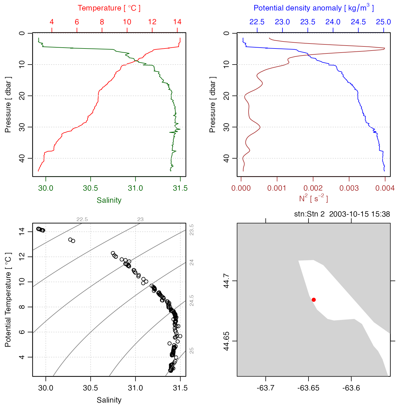
Plot CTD data in any of many different ways. In many cases, the best choice is to use default values for all parameters other than the first. This yields a 4-panel plot that displays a basic overview of the data, with a combined profile of salinity and temperature at the top left, a combined plot of density and the square of buoyancy frequency at top right, a TS diagram at bottom left, and a map at bottom right.

# S4 method for ctd
plot(
  x,
  which,
  col = par("fg"),
  fill,
  borderCoastline = NA,
  colCoastline = "lightgray",
  eos = getOption("oceEOS", default = "gsw"),
  ref.lat = NaN,
  ref.lon = NaN,
  grid = TRUE,
  coastline = "best",
  Slim,
  Clim,
  Tlim,
  plim,
  densitylim,
  sigmalim,
  N2lim,
  Rrholim,
  dpdtlim,
  timelim,
  drawIsobaths = FALSE,
  clongitude,
  clatitude,
  span,
  showHemi = TRUE,
  lonlabels = TRUE,
  latlabels = TRUE,
  latlon.pch = 20,
  latlon.cex = 1.5,
  latlon.col = "red",
  projection = NULL,
  cex = 1,
  cex.axis = par("cex.axis"),
  pch = 1,
  useSmoothScatter = FALSE,
  df,
  keepNA = FALSE,
  type,
  mgp = getOption("oceMgp"),
  mar = c(mgp[1] + 1.5, mgp[1] + 1.5, mgp[1] + 1.5, mgp[1] + 1),
  inset = FALSE,
  add = FALSE,
  debug = getOption("oceDebug"),
  ...
)

Arguments

x

a ctd object.

which

a numeric or character vector specifying desired plot types. If which is not supplied, a default will be used. This default depends on deploymentType in the metadata slot of x. If deploymentType is "profile" or missing, then which defaults to c(1, 2, 3, 5). If deploymentType is "moored" or "thermosalinograph" then which defaults to c(30, 3, 31, 5). Finally, if deploymentType is towyo then which defaults to c(30, 31, 32, 3).

The details of individual which values are as follows. Some of the entries refer to the EOS (equation of state for seawater), which may either "gsw" for the modern Gibbs Seawater system, or "unesco" for the older UNESCO system. The EOS may be set with the eos argument to plot,ctd-method() or by using options(), with options(oceEOS="unesco") or options(oceEOS="unesco"). The default EOS is "gsw".

which=1 or which="salinity+temperature" gives a combined profile of temperature and salinity. If the EOS is "gsw" then Conservative Temperature and Absolute Salinity are shown; otherwise in-situ temperature and practical salinity are shown.
which=2 or which="density+N2" gives a combined profile of density anomaly, computed with swSigma0(), along with the square of the buoyancy frequency, computed with swN2(). The eos parameter is passed to each of these functions, so the desired EOS is used.
which=3 or which="TS" gives a TS plot. If the EOS is "gsw", T is Conservative Temperature and S is Absolute Salinity; otherwise, they are in-situ temperature and practical salinity, respectively.
which=4 or which="text" gives a textual summary of some aspects of the data.
which=5 or which="map" gives a map plotted with plot,coastline-method(), with a dot for the station location. Notes near the top boundary of the map give the station number, the sampling date, and the name of the chief scientist, if these are known. Note that the longitude will be converted to a value between -180 and 180 before plotting. (See also notes about span.)
which=5.1 as for which=5, except that the file name is drawn above the map.
which=6 or which="density+dpdt" gives a profile of density and \(dP/dt\), which is useful for evaluating whether the instrument is dropping properly through the water column. If the EOS is "gsw" then \(\sigma_0\) is shown; otherwise, \(\sigma_\theta\) is shown.
which=7 or which="density+time" gives a profile of density and time.
which=8 or which="index" gives a profile of index number, which can provide useful information for trimming with ctdTrim().
which=9 or which="salinity" gives a profile of Absolute Salinity if the EOS is "gsw", or practical salinity otherwise.
which=10 or which="temperature" gives a profile of Conservative Temperature if the EOS is "gsw", or in-situ temperature otherwise.
which=11 or which="density" gives a profile of density as computed with swRho(), to which the eos parameter is passed.
which=12 or which="N2" gives an \(N^2\) profile.
which=13 or which="spice" gives a profile of the UNESCO-defined spice variable.
which=14 or which="tritium" gives a tritium profile.
which=15 or which="Rrho" gives a diffusive-case density ratio profile.
which=16 or which="RrhoSF" gives a salt-finger case density ratio profile.
which=17 or which="conductivity" gives a conductivity profile.
which=20 or which="CT" gives a profile of Conservative Temperature.
which=21 or which="SA" gives a profile of Absolute Salinity.
which=30 or which="Sts" gives a time series of Salinity Absolute Salinity if the EOS is "gsw" or practical salinity otherwise.
which=31 or which="Tts" gives a time series of Conservative Temperature if the EOS is "gsw" or in-situ temperature otherwise.
which=32 or which="pts" gives a time series of pressure
which=33 or which="rhots" gives a time series of density anomaly, \(\sigma_0\) if the EOS is "gsw" or \(\sigma_\theta\) otherwise.
otherwise, which is interpreted as a character value to be checked against the data and dataDerived fields returned by x[["?"]. If a match is found then a profile of the corresponding quantity is plotted. If there is no match, an error is reported.

col

color of lines or symbols.

fill

a legacy parameter that will be permitted only temporarily; see “History”.

borderCoastline

color of coastlines and international borders, passed to plot,coastline-method() if a map is included in which.

colCoastline

fill color of coastlines and international borders, passed to plot,coastline-method() if a map is included in which. Set to NULL to avoid filling.

eos

character value indicating the equation of state to be used, either "unesco" or "gsw". The default is to use a value stored with options() as e.g. options(oceEOS="unesco").

ref.lat

latitude of reference point for distance calculation. The permitted range is -90 to 90.

ref.lon

longitude of reference point for distance calculation. The permitted range is -180 to 180.

grid

logical value indicating whether to draw a grid on the plot.

coastline

a specification of the coastline to be used for which="map". This may be a coastline object, whether built-in or supplied by the user, or a character string. If the later, it may be the name of a built-in coastline ("coastlineWorld", "coastlineWorldFine", or "coastlineWorldCoarse"), or "best", to choose a suitable coastline for the locale, or "none" to prevent the drawing of a coastline. There is a speed penalty for providing coastline as a character string, because it forces plot,coastline-method() to load it on every call. So, if plot,coastline-method() is to be called several times for a given coastline, it makes sense to load it in before the first call, and to supply the object as an argument, as opposed to the name of the object.

Slim, Clim, Tlim, plim, densitylim, sigmalim, N2lim, Rrholim, dpdtlim, timelim

optional numeric vectors of length 2, that give axis limits for salinity (or Absolute Salinity, if eos is "gsw"), conductivity, in-situ or potential temperature (or Conservative Temperature, if eos is `"gsw"'), pressure, density, density anomaly (either sigma-theta or sigma0), square of buoyancy frequency, density ratio, dp/dt, and time, respectively.

drawIsobaths

logical value indicating whether to draw depth contours on maps, in addition to the coastline. The argument has no effect except for panels in which the value of which equals "map" or the equivalent numerical code, 5. If drawIsobaths is FALSE, then no contours are drawn. If drawIsobaths is TRUE, then contours are selected automatically, using pretty(c(0, 300)) if the station depth is under 100m or pretty(c(0, 5500)) otherwise. If drawIsobaths is a numerical vector, then the indicated depths are drawn. For plots drawn with projection set to NULL, the contours are added with contour() and otherwise mapContour() is used. To customize the resultant contours, e.g. setting particular line types or colors, users should call these functions directly (see e.g. Example 2).

clongitude, clatitude, span

controls for the map area view, used only if which="map". clongitude and clatitude specify the centre of the view, and span specifies the approximate extend of the view, in kilometres. (If span is not given, it is be determined as a small multiple of the distance to the nearest point of land, in an attempt to show the station in familiar geographical context.)

showHemi, lonlabels, latlabels

controls for axis labelling, used only if which="map". showHemi is logical value indicating whether to show hemisphere in axis tick labels. lonlabels and latlabels are numeric and character values that control the axis labelling.

latlon.pch, latlon.cex, latlon.col

controls for station location, used only if which="map". latlon.pch sets the symbol code, latlon.cex sets the character expansion factor, and latlon.col sets the colour.

projection

controls the map projection (if any), and ignored unless which="map". The possibilities are as follows. (1) If projection=NULL (the default) then no projection will be used; the map will simply show longitude and latitude in a Cartesian frame, scaled to retain shapes at the centre. (2) If projection="automatic"then either a Mercator or Stereographic projection will be used, depending on whether the CTD station is within 70 degrees of the equator or at higher latitudes. (3) Ifprojection` is a string in the format used by mapPlot(), then it is is passed to that function.

cex

size to be used for plot symbols (see par()).

cex.axis

size factor for axis labels (see par()).

pch

code for plotting symbol (see par()).

useSmoothScatter

logical value indicating whether to use smoothScatter() instead of plot() to draw the plot.

df

optional numeric argument that is ignored except for plotting buoyancy frequency; in that case, it is passed to swN2().

keepNA

logical value indicating whether NA values will yield breaks in lines drawn if type is b, l, or o. The default value is FALSE. Setting keepNA to TRUE can be helpful when working with multiple profiles strung together into one ctd object, which otherwise would have extraneous lines joining the deepest point in one profile to the shallowest in the next profile.

type

the type of plot to draw, using the same scheme as plot(). If supplied, this is increased to be the same length as which, if necessary, and then supplied to each of the individual plot calls. If it is not supplied, then those plot calls use defaults (e.g. using a line for plotProfile(), using dots for plotTS(), etc).

mgp

three-element numerical vector specifying axis-label geometry, passed to par(). The default establishes tighter margins than in the usual R setup.

mar

four-element numerical vector specifying margin geometry, passed to par(). The default establishes tighter margins than in the usual R setup. Note that the value of mar is ignored for the map panel of multi-panel maps; instead, the present value of par("mar") is used, which in the default call will make the map plot region equal that of the previously-drawn profiles and TS plot.

inset

logical value indicating whether this function is being used as an inset. The effect is to prevent the present function from adjusting margins, which is necessary because margin adjustment is the basis for the method used by plotInset().

add

logical value indicating whether to add to an existing plot. This only works if length(which)=1, and it will yield odd results if the value of which does not match that in the previous plots.

debug

an integer specifying whether debugging information is to be printed during the processing. This is a general parameter that is used by many oce functions. Generally, setting debug=0 turns off the printing, while higher values suggest that more information be printed. If one function calls another, it usually reduces the value of debug first, so that a user can often obtain deeper debugging by specifying higher debug values.

...

optional arguments passed to plotting functions.

Details

The default values of which and other arguments are chosen to be useful for quick overviews of data. However, for detailed work it is common to call the present function with just a single value of which, e.g. with four calls to get four panels. The advantage of this is that it provides much more control over the display, and also it permits the addition of extra display elements (lines, points, margin notes, etc.) to the individual panels.

Note that panels that draw more than one curve (e.g. which="salinity+temperature" draws temperature and salinity profiles in one graph), the value of par("usr") is established by the second profile to have been drawn. Some experimentation will reveal what this profile is, for each permitted which case, although it seems unlikely that this will help much ... the simple fact is that drawing two profiles in one graph is useful for a quick overview, but not useful for e.g. interactive analysis with locator() to flag bad data, etc.

History of Changes

January 2022:
- Add ability to profile anything stored in the data slot, and anything that can be computed from information in that slot. The list of possibilities is found by examining the data and dataDerived elements of x[["?"]].
- Drop the lonlim and latlim parameters, marked for removal in 2014; use clongitude, clatitude and span instead (see plot,coastline-method()).
February 2016:
- Drop the fill parameter for land colour; use colCoastline instead.
- Add the borderCoastline argument, to control the colour of coastlines and international boundaries.

Author

Dan Kelley

Examples

# 1. simple plot
library(oce)
data(ctd)
plot(ctd)


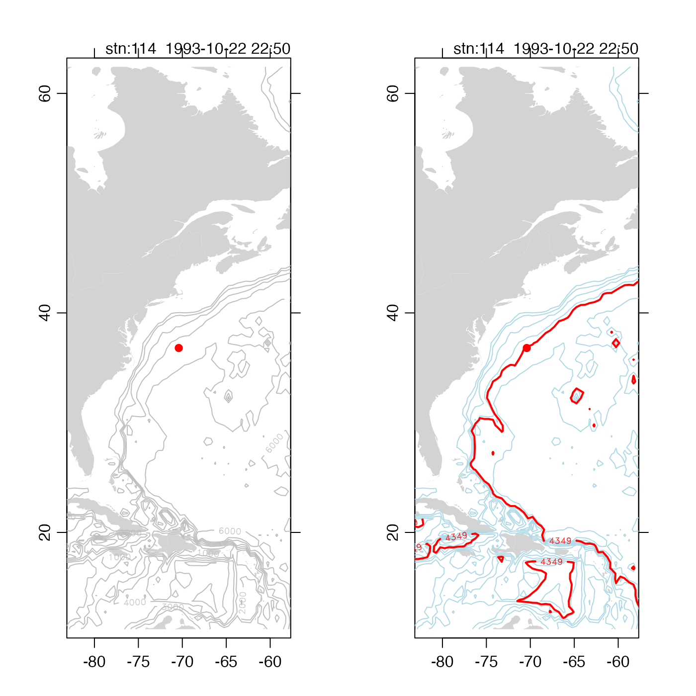
# 2. how to customize depth contours
par(mfrow = c(1, 2))
data(section)
stn <- section[["station", 105]]
plot(stn, which = "map", drawIsobaths = TRUE)
plot(stn, which = "map")
data(topoWorld)
tlon <- topoWorld[["longitude"]]
tlat <- topoWorld[["latitude"]]
tdep <- -topoWorld[["z"]]
contour(tlon, tlat, tdep,
    drawlabels = FALSE,
    levels = seq(1000, 6000, 1000), col = "lightblue", add = TRUE
)
contour(tlon, tlat, tdep,
    vfont = c("sans serif", "bold"),
    levels = stn[["waterDepth"]], col = "red", lwd = 2, add = TRUE
)

Arguments

Details

History of Changes

See also

Author

Examples