Add a Grid to an Existing Oce Plot
Usage
oce.grid(xat, yat, col = "lightgray", lty = "dotted", lwd = par("lwd"))Arguments
- xat
either a list of x values at which to draw the grid, or the return value from an oce plotting function
- yat
a list of y values at which to plot the grid (ignored if
gxwas a return value from an oce plotting function)- col
color of grid lines (see
par())- lty
type for grid lines (see
par())- lwd
width for grid lines (see
par())
Details
For plots not created by oce functions, or for missing xat and yat,
this is the same as a call to grid() with missing nx and
ny. However, if xat is the return value from certain oce functions,
a more sophisticated grid is constructed. The problem with grid() is
that it cannot handle axes with non-uniform grids, e.g. those with time axes
that span months of differing lengths.
As of early February 2015, oce.grid handles xat produced as the
return value from the following functions: imagep() and
oce.plot.ts(), plot,adp-method(),
plot,echosounder-method(), and plotTS().
It makes no sense to try to use oce.grid for multipanel oce plots,
e.g. the default plot from plot,adp-method().
Examples
library(oce)
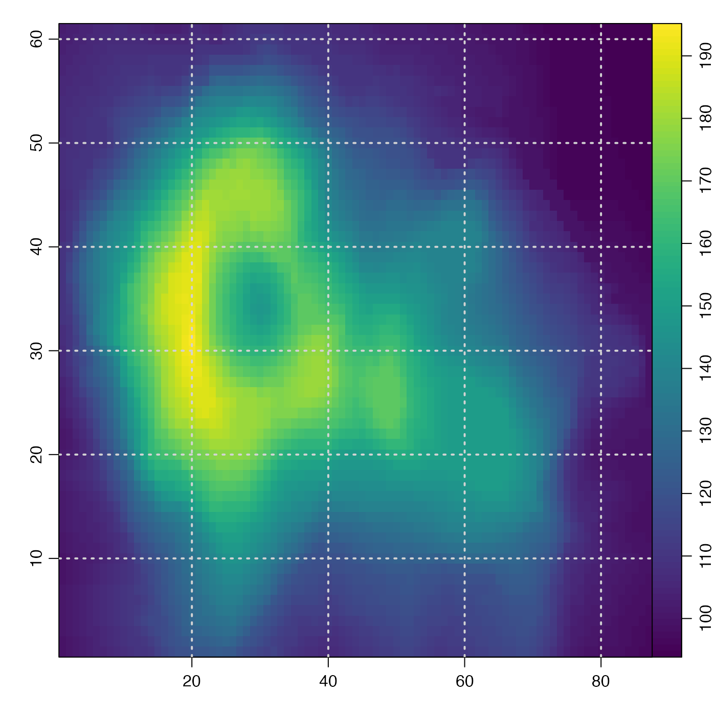
i <- imagep(volcano)
oce.grid(i, lwd = 2)
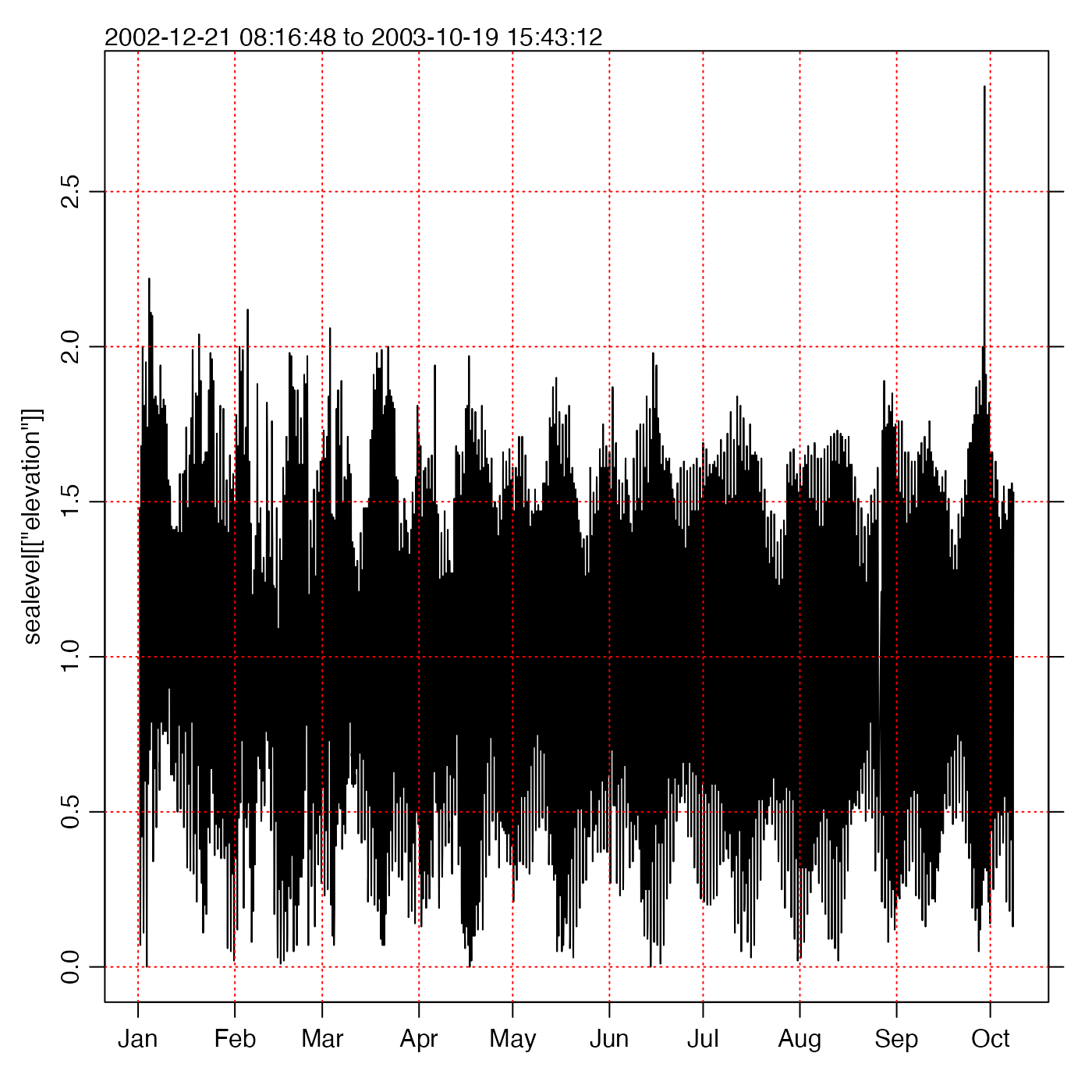
 data(sealevel)
i <- oce.plot.ts(sealevel[["time"]], sealevel[["elevation"]])
oce.grid(i, col = "red")
data(sealevel)
i <- oce.plot.ts(sealevel[["time"]], sealevel[["elevation"]])
oce.grid(i, col = "red")
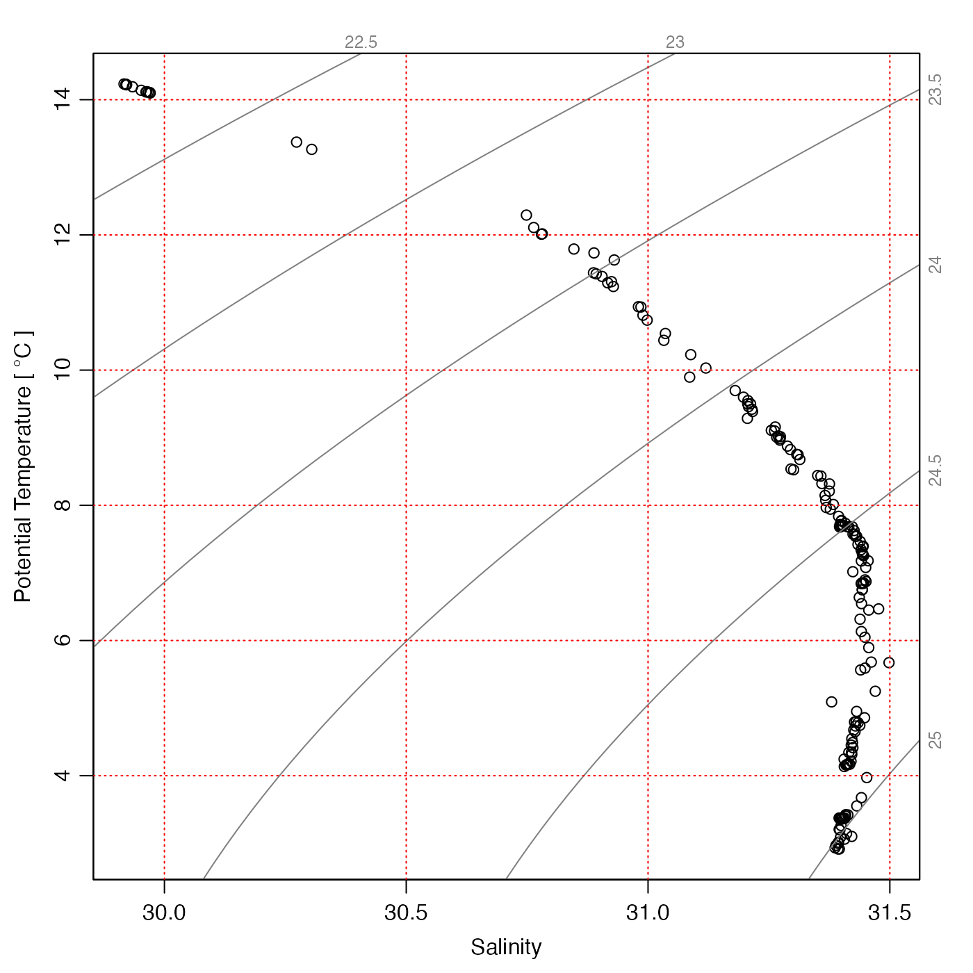
 data(ctd)
i <- plotTS(ctd)
oce.grid(i, col = "red")
data(ctd)
i <- plotTS(ctd)
oce.grid(i, col = "red")
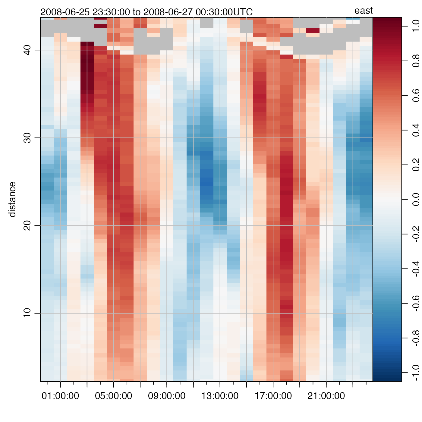
 data(adp)
i <- plot(adp, which = 1)
oce.grid(i, col = "gray", lty = 1)
data(adp)
i <- plot(adp, which = 1)
oce.grid(i, col = "gray", lty = 1)
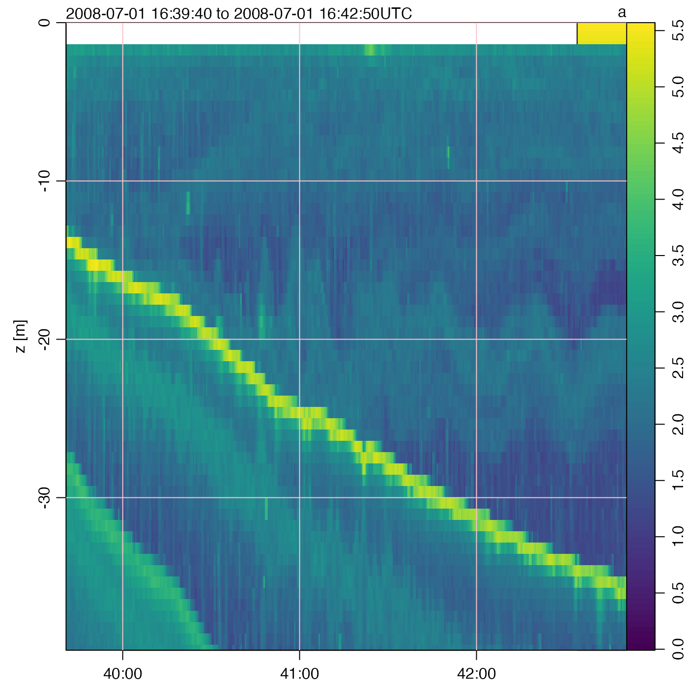
 data(echosounder)
i <- plot(echosounder)
oce.grid(i, col = "pink", lty = 1)
data(echosounder)
i <- plot(echosounder)
oce.grid(i, col = "pink", lty = 1)