Plot a section Object

Creates a summary plot for a CTD section, with one panel for each value of which.

Usage

# S4 method for class 'section'
plot(
  x,
  which,
  eos,
  at = NULL,
  labels = TRUE,
  grid = FALSE,
  contourLevels = NULL,
  contourLabels = NULL,
  stationIndices,
  coastline = "best",
  colLand = "gray",
  xlim = NULL,
  ylim = NULL,
  zlim = NULL,
  zbreaks = NULL,
  zcol = NULL,
  map.xlim = NULL,
  map.ylim = NULL,
  clongitude,
  clatitude,
  span,
  projection = NULL,
  xtype = "distance",
  ytype = "depth",
  ztype = "contour",
  longitude0,
  latitude0,
  legend.loc = "bottomright",
  legend.text = NULL,
  showStations = FALSE,
  showStart = TRUE,
  stationTicks = TRUE,
  showBottom = TRUE,
  showSpine = TRUE,
  drawPalette = TRUE,
  axes = TRUE,
  mgp,
  mar,
  col,
  cex,
  pch,
  lwd,
  labcex = par("cex"),
  debug = getOption("oceDebug", 0),
  ...
)

Arguments

x: a section object.
which: a list of desired plot types, as explained in “Details”. Plot types not listed in “Details” can be generated using the name of the data in the section object. There may be up to four panels in total, and the desired plots are placed in these panels, in reading order. If only one panel is plotted, par is not adjusted, which makes it easy to add to the plot with subsequent plotting commands.
eos: Character indication of the seawater equation of state to use. The permitted choices are "gsw" and "unesco". If eos is not supplied, it defaults to getOption("oceEOS",default="gsw").
at: If NULL (the default), the x axis will indicate the distance of the stations from the first in the section. (This may give errors in the contouring routine, if the stations are not present in a geographical order.) If a list, then it indicates the values at which stations will be plotted.
labels: Either a logical, indicating whether to put labels on the x axis, or a vector that is a list of labels to be placed at the x positions indicated by at.
grid: If TRUE, points are drawn at data locations.
contourLevels: Optional contour levels.
contourLabels: Optional contour labels.
stationIndices: Optional list of the indices of stations to use. Note that an index is not a station number, e.g. to show the first 4 stations, use station.indices=1:4.
coastline: Either a coastline object to be used, or a string. In the second case, the permitted choices are "best" (the default) to pick a variant that suits the scale, "coastlineWorld" for the coarse version that is provided by oce, "coastlineWorldMedium" or "coastlineWorldFine" for two coastlines provided by the ocedata package, or "none", to avoid drawing a coastline.
colLand: colour used to fill in land areas if which is "map"; ignored otherwise.
xlim: Optional limit for x axis (only in sections, not map).
ylim: Optional limit for y axis (only in sections, not map)
zlim, zbreaks, zcol: Elements that control colours for image and points plot types, i.e. if ztype is either "points" or "image". zlim is a two-element numerical vector specifying the limit on the plotted field. If not provided, it defaults to the data range. zbreaks controls the colour breaks, in a manner that is similar to the image() parameter named breaks. If not provided, zbreaks is inferred from zlim. zcol, which controls the colour scheme, may be a vector of colours (of length 1 less than zbreaks), or a function that takes an integer as its sole argument and returns that number of colours. If not provided, zcol defaults to oceColorsViridis(). These three parameters are used in Example 6, an illustration of Atlantic salinity along 36N.
map.xlim, map.ylim: Optional limits for station map; map.ylim is ignored if map.xlim is provided.
clongitude, clatitude, span: Optional map centre position and span (km).
projection: Parameter specifying map projection; see mapPlot(). If projection="automatic", however, a projection is devised from the data, with stereographic if the mean latitude exceeds 70N and mollweide otherwise.
xtype: Type of x axis, for contour plots, either "distance" for distance (in km) to the first point in the section, "track" for distance along the cruise track, "longitude", "latitude", "time" or "spine" (distance along a spine that was added with addSpine()). Note that if the x values are not in order, they will be put in order, and since that might not make physical sense, a warning will be issued.
ytype: Type of y axis for contour plots, either "pressure" for pressure (in dbar, with zero at the surface) or "depth" for depth (in m below the surface, calculated from pressure with swDepth()).
ztype: String indicating whether to how to indicate the "z" data (in the R sense, i.e. this could be salinity, temperature, etc; it does not mean the vertical coordinate) The choices are: "contour" for contours, "image" for an image (drawn with imagep() with filledContours=TRUE), or "points" to draw points. In the first two cases, the data must be gridded, with identical pressures at each station.
longitude0, latitude0: Location of the point from which distance is measured. These values are ignored unless xtype is "distance".
legend.loc: Location of legend, as supplied to legend(), or set to the empty string to avoid plotting a legend.
legend.text: character value indicating the text for the legend. If this is NULL (the default) then the legend is automatically constructed by labelWithUnit(), based on the value of which.
showStations: Logical indicating whether to draw station numbers on maps.
showStart: Logical indicating whether to indicate the first station with
stationTicks: A logical value indicating whether to indicate station locations with ticks at the top margin of cross-section plots. Setting this parameter to FALSE frees the user up to do their own labelling at this spot.
showBottom: a value indicating whether (and how) to indicate the ocean bottom on cross-section views. There are three possibilities. (a) If showBottom is FALSE, then the bottom is not rendered. If it is TRUE, then the bottom is rendered with a gray polygon. (b) If showBottom is the character value "polygon", then a polygon is drawn, and similarly lines are drawn for "lines", and points for "points". (c) If showBottom is a topo object, then the station locations are interpolated to that topography and the results are shown with a polygon. See “Examples”.
showSpine: logical value used if which="map". If showSpine is TRUE and section has had a spine added with addSpine(), then the spine is drawn in blue.
drawPalette: logical value indicating whether to draw a palette when ztype="image" ignored otherwise.
axes: Logical value indicating whether to draw axes.
mgp: A 3-element numerical vector to use for par(mgp), and also for par(mar), computed from this. If not provided, this defaults to getOption("oceMgp").
mar: Value to be used with par("mar"). If not provided, a default is set up.
col: Color for line types. If not provided, this defaults to par("col"). See zcol, for ztype="image" and ztype="points".
cex: Numerical character-expansion factor, which defaults to par("cex").
pch: Indication of symbol type; defaults to par("pch") for non-map or to 3 for map.
lwd: line width; defaults to par("lwd").
labcex: Size of characters in contour labels (passed to contour()).
debug: an integer specifying whether debugging information is to be printed during the processing. This is a general parameter that is used by many oce functions. Generally, setting debug=0 turns off the printing, while higher values suggest that more information be printed. If debug is not supplied, it defaults to getOption("oceDebug").
...: Optional arguments passed to the contouring function.

Value

If the original section was gridded, the return value is that section. Otherwise, the gridded section that was constructed for the plot is returned. In both cases, the value is returned silently. The purpose of returning the section is to enable subsequent processing of the grid, including adding elements to the plot (see example 5).

Details

The type of plot is governed by which, as listed below; if which is not supplied, it defaults to c(1,2,3,99) if eos is "unesco" or to c(1.5,2.5,3.5,99) if eos is "gsw".

which=0 or "potential temperature" for potential temperature contours
which=1 or "temperature" for in-situ temperature contours
which=1.5 or "CT" for Conservative Temperature contours
which=2 or "salinity" for salinity contours
which=2.5 or "SA" for Absolute Salinity contours
which=3 or "sigmaTheta" for sigma-theta (a unesco variable) contours
which=3.5 or "sigma0" for sigma0 (a gsw variable) contours
which=4 or "nitrate" for nitrate concentration contours
which=5 or "nitrite" for nitrite concentration contours
which=6 or "oxygen" for oxygen concentration contours
which=7 or "phosphate" for phosphate concentration contours
which=8 or "silicate" for silicate concentration contours
which=9 or "u" for eastward velocity
which=10 or "uz" for vertical derivative of eastward velocity
which=11 or "v" for northward velocity
which=12 or "vz" for vertical derivative of northward velocity
which=20 or "data" for a dot for each data location
which=99 or "map" for a location map

The y-axis for the contours is pressure, plotted in the conventional reversed form, so that the water surface appears at the top of the plot. The x-axis is more complicated. If at is not supplied, then the routine calculates x as the distance between the first station in the section and each of the other stations. (This will produce an error if the stations are not ordered geographically, because the contour() routine cannot handle non-increasing axis coordinates.) If at is specified, then it is taken to be the location, in arbitrary units, along the x-axis of labels specified by labels; the way this works is designed to be the same as for axis().

Ancillary Examples

The following examples were once part of the “Examples” section, but were moved here in May 2022, to reduce the build-check time for CRAN submission.

library(oce)
data(section)
GS <- subset(section, 113<=stationId&stationId<=129)
GSg <- sectionGrid(GS, p=seq(0, 2000, 100))

# Gulf Stream, salinity data and contoured
par(mfrow=c(2, 1))
plot(GS, which=1, ylim=c(2000, 0), ztype="points",
     zbreaks=seq(0,30,2), pch=20, cex=3)
plot(GSg, which=1, ztype="image", zbreaks=seq(0,30,2))

# Gulf Stream, temperature grid (image) and data (dots)
par(mfrow=c(1, 1))
plot(GSg, which=1, ztype="image")
T <- GS[["temperature"]]
col <- oceColorsViridis(100)[rescale(T, rlow=1, rhigh=100)]
points(GS[["distance"]],GS[["depth"]],pch=20,cex=3,col="white")
points(GS[["distance"]],GS[["depth"]],pch=20,cex=2.5,col=col)

# 4. Image of temperature, with a high-salinity contour on top;
#    note the Mediterranean water.
sec <- plot(section, which="temperature", ztype="image")
S <- sec[["salinity", "grid:distance-pressure"]]
contour(S$distance, S$pressure, S$field, level=35.8, lwd=3, add=TRUE)

# 5. Contours of salinity, with dots for high pressure and spice
plot(section, which="salinity")
distance <- section[["distance"]]
depth <- section[["depth"]]
spice <- section[["spice"]]
look <- spice > 1.8 & depth > 500
points(distance[look], depth[look], col="red")

# Image of Absolute Salinity, with 4-minute bathymetry
# It's easy to calculate the desired area for the bathymetry,
# but for brevity we'll hard-code it. Note that download.topo()
# requires the "ncdf4" package to have been installed.
if (requireNamespace("ncdf4")) {
    f <- download.topo(west=-80, east=0, south=35, north=40, resolution=4)
    t <- read.topo(f)
    plot(section, which="SA", xtype="longitude", ztype="image", showBottom=t)
}

# Temperature with salinity added in red
plot(GSg, which="temperature")
distance <- GSg[["distance", "byStation"]]
depth <- GSg[["station", 1]][["depth"]]
S <- matrix(GSg[["salinity"]], byrow=TRUE, nrow=length(GSg[["station"]]))
contour(distance, depth, S, col=2, add=TRUE)

# Image with controlled colours
plot(GSg, which="salinity", ztype="image",
    zlim=c(35, 37.5),
    zbreaks=seq(35, 37.5, 0.25),
    zcol=oceColorsTurbo)

Author

Dan Kelley, with help from Clark Richards and Chantelle Layton.

Examples

library(oce)
data(section)
GS <- subset(section, 113 <= stationId & stationId <= 129)
GSg <- sectionGrid(GS, p = seq(0, 2000, 100))

# Gulf Stream, salinity and temperature contours
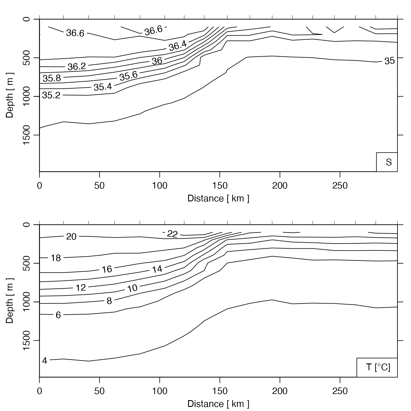
plot(GSg, which = c("salinity", "temperature"))


# Gulf Stream, Temperature image
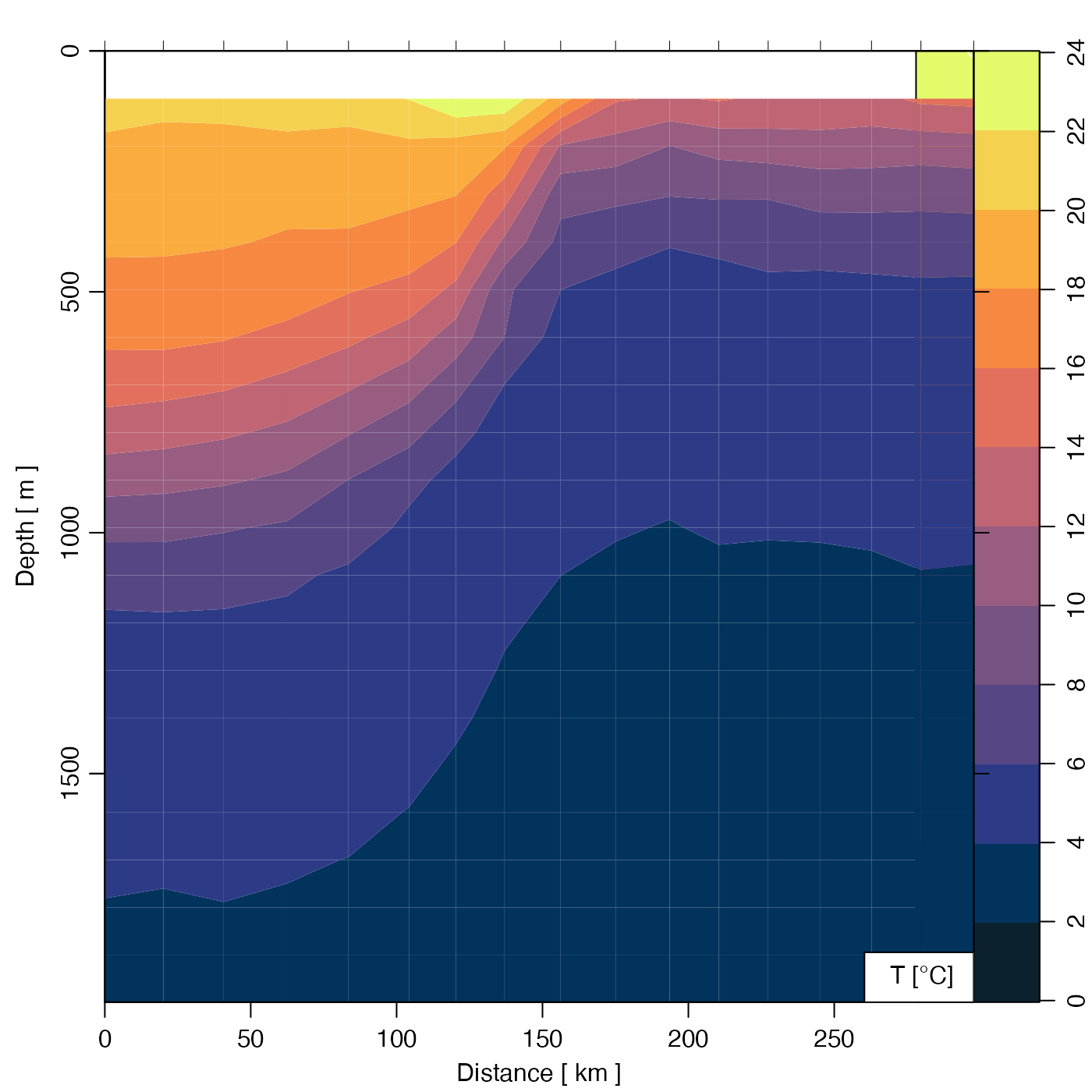
plot(GSg,
    which = "temperature", ztype = "image",
    zbreaks = seq(0, 25, 2), zcol = oceColorsTemperature
)