Plot an Inset Diagram

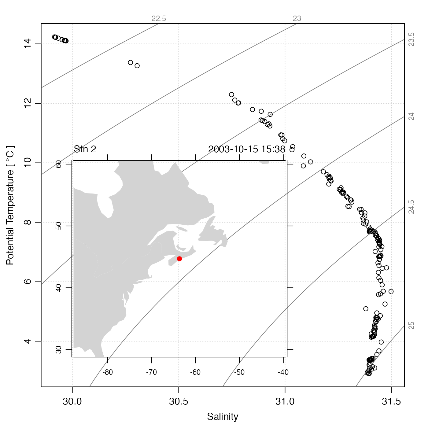
Adds an inset diagram to an existing plot. Note that if the inset is a map or coastline, it will be necessary to supply inset=TRUE to prevent the inset diagram from occupying the whole device width. After plotInset() has been called, any further plotting will take place within the inset, so it is essential to finish a plot before drawing an inset.

Usage

plotInset(
  xleft,
  ybottom,
  xright,
  ytop,
  expr,
  mar = c(2, 2, 1, 1),
  debug = getOption("oceDebug")
)

Arguments

xleft

location of left-hand of the inset diagram, in the existing plot units. (PROVISIONAL FEATURE: this may also be "bottomleft", to put the inset there. Eventually, other positions may be added.)

ybottom

location of bottom side of the inset diagram, in the existing plot units.

xright

location of right-hand side of the inset diagram, in the existing plot units.

ytop

location of top side of the inset diagram, in the existing plot units.

expr

An expression that draws the inset plot. This may be a single plot command, or a sequence of commands enclosed in curly braces.

mar

margins, in line heights, to be used at the four sides of the inset diagram. (This is often helpful to save space.)

debug

a flag that turns on debugging. Set to 1 to get a moderate amount of debugging information, or to 2 to get more.

Author

Dan Kelley

Examples

library(oce)
# power law in linear and log form
x <- 1:10
y <- x^2
plot(x, y, log = "xy", type = "l")
plotInset(3, 1, 10, 8,
    expr = plot(x, y, type = "l", cex.axis = 3 / 4, mgp = c(3 / 2, 1 / 2, 0)),
    mar = c(2.5, 2.5, 1, 1)
)


# CTD data with location
data(ctd)
plot(ctd, which = "TS")
plotInset(29.9, 2.7, 31, 10,
    expr = plot(ctd,
        which = "map",
        coastline = "coastlineWorld",
        span = 5000, mar = NULL, cex.axis = 3 / 4
    )
)