Draw a Map — mapPlot • oce

Plot coordinates as a map, using one of the subset of projections provided by the sf package. The projection information specified with the mapPlot() call is stored in a global variable that can be retrieved by related functions, making it easy to add points, lines, text, images or contours to an existing map. The “Details” section, below, provides a list of available projections. The "Using map projections" vignette offers examples of several map plots, in addition to the single example provided in the “Examples” section.

mapPlot(
  longitude,
  latitude,
  longitudelim,
  latitudelim,
  grid = TRUE,
  geographical = 0,
  bg,
  fill,
  border = NULL,
  col = NULL,
  clip = TRUE,
  type = "polygon",
  axes = TRUE,
  axisStyle = 1,
  cex,
  cex.axis = 1,
  mgp = c(0, 0.5, 0),
  drawBox = TRUE,
  showHemi = TRUE,
  polarCircle = 0,
  lonlabels = TRUE,
  latlabels = TRUE,
  projection = "+proj=moll",
  tissot = FALSE,
  trim = TRUE,
  debug = getOption("oceDebug"),
  ...
)

Arguments

longitude: either a numeric vector of longitudes of points to be plotted, or something (an oce object, a list, or a data frame) from which both longitude and latitude may be inferred (in which case the latitude argument is ignored). If longitude is missing, both it and latitude are taken from the built-in coastlineWorld dataset.
latitude: numeric vector of latitudes of points to be plotted (ignored if the first argument contains both latitude and longitude).
longitudelim, latitudelim: optional numeric vectors of length two, indicating the limits of the plot. A warning is issued if these are not specified together. See “Examples” for a polar-region example, noting that the whole-globe span of longitudelim is used to centre the plot at the north pole.
grid: either a number (or pair of numbers) indicating the spacing of longitude and latitude lines, in degrees, or a logical value (or pair of values) indicating whether to draw an auto-scaled grid, or whether to skip the grid drawing. In the case of numerical values, NA can be used to turn off the grid in longitude or latitude. Grids are set up based on examination of the scale used in middle 10 percent of the plot area, and for most projections this works quite well. If not, one may set grid=FALSE and add a grid later with mapGrid().
geographical: flag indicating the style of axes. With geographical=0, the axes are conventional, with decimal degrees as the unit, and negative signs indicating the southern and western hemispheres. With geographical=1, the signs are dropped, with axis values being in decreasing order within the southern and western hemispheres. With geographical=2, the signs are dropped and the axes are labelled with degrees, minutes and seconds, as appropriate, and hemispheres are indicated with letters. With geographical=3, things are the same as for geographical=2, but the hemisphere indication is omitted. Finally, with geographical=4, unsigned numbers are used, followed by letters N in the northern hemisphere, S in the southern, E in the eastern, and W in the western.
bg: color of the background (ignored).
fill: is a deprecated argument; see oce-deprecated.
border: color of coastlines and international borders (ignored unless type="polygon".
col: either the color for filling polygons (if type="polygon") or the color of the points and line segments (if type="p", type="l", or type="o"). If col=NULL then a default will be set: no coastline filling for the type="polygon" case, or black coastlines, for type="p", type="l", or type="o".
clip: logical value indicating whether to trim any coastline elements that lie wholly outside the plot region. This can prevent e.g. a problem of filling the whole plot area of an Arctic stereopolar view, because the projected trace for Antarctica lies outside all other regions so the whole of the world ends up being "land". Setting clip=FALSE disables this action, which may be of benefit in rare instances in the line connecting two points on a coastline may cross the plot domain, even if those points are outside that domain.
type: indication of type; may be "polygon", for a filled polygon, "p" for points, "l" for line segments, or "o" for points overlain with line segments.
axes: a logical value indicating whether to draw longitude and latitude values in the lower and left margin, respectively. This may not work well for some projections or scales. See also axisStyle, lonlabels and latlabels, which offer more granular control of labelling.
axisStyle: an integer specifying the style of labels for the numbers on axes. The choices are: 1 for signed numbers without additional labels; 2 (the default) for unsigned numbers followed by letters indicating the hemisphere; 3 for signed numbers followed by a degree sign; 4 for unsigned numbers followed by a degree sign; and 5 for signed numbers followed by a degree sign and letters indicating the hemisphere.
cex: character expansion factor for plot symbols, used if type="p" or any other value that yields symbols.
cex.axis: axis-label expansion factor (see par()).
mgp: three-element numerical vector describing axis-label placement, passed to mapAxis().
drawBox: logical value indicating whether to draw a box around the plot. This is helpful for many projections at sub-global scale.
showHemi: logical value indicating whether to show the hemisphere in axis tick labels.
polarCircle: a number indicating the number of degrees of latitude extending from the poles, within which zones are not drawn.
lonlabels: An optional logical value or numeric vector that controls the labelling along the horizontal axis. There are four possibilities: (1) If lonlabels is TRUE (the default), then reasonable values are inferred and axes are drawn with ticks and labels alongside those ticks; (2) if lonlabels is FALSE, then ticks are drawn, but no labels; (3) if lonlabels is NULL, then no axis ticks or labels are drawn; and (4) if lonlabels is a vector of finite numerical values, then tick marks are placed at those longitudes, and labels are put alongside them. Note that R tries to avoid overwriting labels on axes, so the instructions in case 4 might not be obeyed exactly. See also latlabels, and note that setting axes=FALSE ensures that no longitude or latitude axes will be drawn regardless of the values of lonlabels and latlabels.
latlabels: As lonlabels, but for latitude, on the left plot axis.
projection: either character value indicating the map projection, or the output from sf::st_crs(). In the first case, see a table in “Details” for the projections that are available. In the second case, note that mapPlot() reports an error if a similar function from the old sp package is used.
tissot: logical value indicating whether to use mapTissot() to plot Tissot indicatrices, i.e. ellipses at grid intersection points, which indicate map distortion.
trim: logical value indicating whether to trim islands or lakes containing only points that are off-scale of the current plot box. This solves the problem of Antarctica overfilling the entire domain, for an Arctic-centred stereographic projection. It is not a perfect solution, though, because the line segment joining two off-scale points might intersect the plotting box.
debug: a flag that turns on debugging. Set to 1 to get a moderate amount of debugging information, or to 2 to get more.
...: optional arguments passed to some plotting functions. This can be useful in many ways, e.g. Example 5 shows how to use xlim etc to reproduce a scale exactly between two plots.

Details

The calculations for map projections are done with the sf package. Importantly, though, not all the sf projections are available in oce, for reasons relating to limitations of sf, for example relating to inverse-projection calculations. The oce choices are tabulated below, e.g. projection="+proj=aea" selects the Albers equal area projection. (See also the warning, below, about a problem with sf version 0.9-8.)

Further details of the vast array of map projections are given in reference 4. This system has been in rapid development since about 2018, and reference 5 provides a helpful overview of the changes and the reasons why they were necessary. Practical examples of map projections in oce are provided in reference 6, along with some notes on problems. A fascinating treatment of the history of map projections is provided in reference 7. To get an idea of how projections are being created nowadays, see reference 8, about the eqearth projection that was added to oce in August 2020.

Available Projections

The following table lists projections available in oce, and was generated by reformatting a subset of the output of the unix command proj -lP. Most of the arguments have default values, and many projections also have optional arguments. Although e.g. proj -l=aea provides a little more information about particular projections, users ought to consult reference 4 for fuller details and illustrations.

Projection	Code	Arguments
Albers equal area	`aea`	`lat_1`, `lat_2`
Azimuthal equidistant	`aeqd`	`lat_0`, `guam`
Aitoff	`aitoff`	-
Mod. stererographics of Alaska	`alsk`	-
Bipolar conic of western hemisphere	`bipc`	-
Bonne Werner	`bonne`	`lat_1`
Cassini	`cass`	-
Central cylindrical	`cc`	-
Equal area cylindrical	`cea`	`lat_ts`
Collignon	`collg`	-
Craster parabolic Putnins P4	`crast`	-
Eckert I	`eck1`	-
Eckert II	`eck2`	-
Eckert III	`eck3`	-
Eckert IV	`eck4`	-
Eckert V	`eck5`	-
Eckert VI	`eck6`	-
Equidistant cylindrical plate (Caree)	`eqc`	`lat_ts`, `lat_0`
Equidistant conic	`eqdc`	`lat_1`, `lat_2`
Equal earth	`eqearth`	-
Euler	`euler`	`lat_1`, `lat_2`
Extended transverse Mercator	`etmerc`	-
Fahey	`fahey`	-
Foucault	`fouc`	-
Foucault sinusoidal	`fouc_s`	-
Gall stereographic	`gall`	-
Geostationary satellite view	`geos`	`h`
General sinusoidal series	`gn_sinu`	`m`, `n`
Gnomonic	`gnom`	-
Goode homolosine	`goode`	-
Hatano asymmetrical equal area	`hatano`	-
Interrupted Goode homolosine	`igh`	-
Kavraisky V	`kav5`	-
Kavraisky VII	`kav7`	-
Lambert azimuthal equal area	`laea`	-
Longitude and latitude	`longlat`	-
Longitude and latitude	`latlong`	-
Lambert conformal conic	`lcc`	`lat_1`, `lat_2` or `lat_0`, `k_0`
Lambert equal area conic	`leac`	`lat_1`, `south`
Loximuthal	`loxim`	-
Space oblique for Landsat	`lsat`	`lsat`, `path`
McBryde-Thomas flat-polar sine, no. 1	`mbt_s`	-
McBryde-Thomas flat-polar sine, no. 2	`mbt_fps`	-
McBryde-Thomas flat-polar parabolic	`mbtfpp`	-
McBryde-Thomas flat-polar quartic	`mbtfpq`	-
McBryde-Thomas flat-polar sinusoidal	`mbtfps`	-
Mercator	`merc`	`lat_ts`
Miller oblated stereographic	`mil_os`	-
Miller cylindrical	`mill`	-
Mollweide	`moll`	-
Murdoch I	`murd1`	`lat_1`, `lat_2`
Murdoch II	`murd2`	`lat_1`, `lat_2`
murdoch III	`murd3`	`lat_1`, `lat_2`
Natural earth	`natearth`	-
Nell	`nell`	-
Nell-Hammer	`nell_h`	-
Near-sided perspective	`nsper`	`h`
New Zealand map grid	`nzmg`	-
General oblique transformation	`ob_tran`	`o_proj`, `o_lat_p`, `o_lon_p`,
		`o_alpha`, `o_lon_c`, `o_lat_c`,
		`o_lon_1`, `o_lat_1`,
		`o_lon_2`, `o_lat_2`
Oblique cylindrical equal area	`ocea`	`lat_1`, `lat_2`, `lon_1`, `lon_2`
Oblated equal area	`oea`	`n`, `m`, `theta`
Oblique Mercator	`omerc`	`alpha`, `gamma`, `no_off`,
		`lonc`, `lon_1`, `lat_1`,
		`lon_2`, `lat_2`
Orthographic	`ortho`	-
Polyconic American	`poly`	-
Putnins P1	`putp1`	-
Putnins P2	`putp2`	-
Putnins P3	`putp3`	-
Putnins P3'	`putp3p`	-
Putnins P4'	`putp4p`	-
Putnins P5	`putp5`	-
Putnins P5'	`putp5p`	-
Putnins P6	`putp6`	-
Putnins P6'	`putp6p`	-
Quartic authalic	`qua_aut`	-
Quadrilateralized spherical cube	`qsc`	-
Robinson	`robin`	-
Roussilhe stereographic	`rouss`	-
Sinusoidal aka Sanson-Flamsteed	`sinu`	-
Swiss. oblique Mercator	`somerc`	-
Stereographic	`stere`	`lat_ts`
Oblique stereographic alternative	`sterea`	-
Transverse cylindrical equal area	`tcea`	-
Tissot	`tissot`	`lat_1`, `lat_2`
Transverse Mercator	`tmerc`	`approx`
Two point equidistant	`tpeqd`	`lat_1`, `lon_1`, `lat_2`, `lon_2`
Tilted perspective	`tpers`	`tilt`, `azi`, `h`
Universal polar stereographic	`ups`	`south`
Urmaev flat-polar sinusoidal	`urmfps`	`n`
Universal transverse Mercator	`utm`	`zone`, `south`, `approx`
van der Grinten I	`vandg`	-
Vitkovsky I	`vitk1`	`lat_1`, `lat_2`
Wagner I Kavraisky VI	`wag1`	-
Wagner II	`wag2`	-
Wagner III	`wag3`	`lat_ts`
Wagner IV	`wag4`	-
Wagner V	`wag5`	-
Wagner VI	`wag6`	-
Werenskiold I	`weren`	-
Winkel I	`wink1`	`lat_ts`
Winkel Tripel	`wintri`	`lat_ts`

Choosing a projection

The best choice of projection depends on the application. Users may find projection="+proj=moll" useful for world-wide plots, ortho for hemispheres viewed from the equator, stere for polar views, lcc for wide meridional ranges in mid latitudes, merc in limited-area cases where angle preservation is important, or either aea or eqearth (on local and global scales, respectively) where area preservation is important. The choice becomes more important, the larger the size of the region represented. When it comes to publication, it can be sensible to use the same projection as used in previous reports.

Problems

Map projection is a complicated matter that is addressed here in a limited and pragmatic way. For example, mapPlot tries to draw axes along a box containing the map, instead of trying to find spots along the ``edge'' of the map at which to put longitude and latitude labels. This design choice greatly simplifies the coding effort, freeing up time to work on issues regarded as more pressing. Chief among those issues are (a) the occurrence of horizontal lines in maps that have prime meridians (b) inaccurate filling of land regions that (again) occur with shifted meridians and (c) inaccurate filling of Antarctica in some projections. Generally, issues are tackled first for commonly used projections, such as those used in the examples.

Historical Notes

2020-12-24: complete switch from rgdal to sf, removing the testing scheme created on 2020-08-03.
2020-08-03: added support for the eqearth projection (like robin but an equal-area method).
2020-08-03: dropped support for the healpix, pconic and rhealpix projections, which caused errors with the sf package. (This is not a practical loss, since these interrupted projections were handled badly by mapPlot() in any case.)
2020-08-03: switch from rgdal to sf for calculations related to map projection, owing to some changes in the former package that broke oce code. (To catch problems, oce was set up to use both packages temporarily, issuing warnings if the results differed by more than 1 metre in easting or northing values.)
2017-11-19: imw_p removed, because it has problems doing inverse calculations. This is a also problem in the standalone PROJ.4 application version 4.9.3, downloaded and built on OSX. See https://github.com/dankelley/oce/issues/1319 for details.
2017-11-17: lsat removed, because it does not work in rgdal or in the latest standalone PROJ.4 application. This is a also problem in the standalone PROJ.4 application version 4.9.3, downloaded and built on OSX. See https://github.com/dankelley/oce/issues/1337 for details.
2017-09-30: lcca removed, because its inverse was wildly inaccurate in a Pacific Antarctic-Alaska application (see https://github.com/dankelley/oce/issues/1303).

Sample of Usage


# Example 1.
# Mollweide (referenc 1 page 54) is an equal-area projection that works well
# for whole-globe views.
mapPlot(coastlineWorld, projection="+proj=moll", col="gray")
mtext("Mollweide", adj=1)

# Example 2.
# Note that filling is not employed (`col` is not
# given) when the prime meridian is shifted, because
# this causes a problem with Antarctica
cl180 <- coastlineCut(coastlineWorld, lon_0=-180)
mapPlot(cl180, projection="+proj=moll +lon_0=-180")
mtext("Mollweide with coastlineCut", adj=1)

# Example 3.
# Orthographic projections resemble a globe, making them attractive for
# non-technical use, but they are neither conformal nor equal-area, so they
# are somewhat limited for serious use on large scales.  See Section 20 of
# reference 1. Note that filling is not employed because it causes a problem with
# Antarctica.
if (utils::packageVersion("sf") != "0.9.8") {
    # sf version 0.9-8 has a problem with this projection
    par(mar=c(3, 3, 1, 1))
    mapPlot(coastlineWorld, projection="+proj=ortho +lon_0=-180")
    mtext("Orthographic", adj=1)
}

# Example 4.
# The Lambert conformal conic projection is an equal-area projection
# recommended by reference 1, page 95, for regions of large east-west extent
# away from the equator, here illustrated for the USA and Canada.
par(mar=c(3, 3, 1, 1))
mapPlot(coastlineCut(coastlineWorld, -100),
    longitudelim=c(-130,-55), latitudelim=c(35, 60),
    projection="+proj=lcc +lat_0=30 +lat_1=60 +lon_0=-100", col="gray")
mtext("Lambert conformal", adj=1)

# Example 5.
# The stereographic projection (reference 1, page 120) in the standard
# form used NSIDC (National Snow and Ice Data Center) for the Arctic.
# (See "A Guide to NSIDC's Polar Stereographic Projection" at
# https://nsidc.org/data/user-resources/help-center.)
# Note how the latitude limit extends 20 degrees past the pole,
# symmetrically.
par(mar=c(3, 3, 1, 1))
mapPlot(coastlineWorld,
    longitudelim=c(-180, 180), latitudelim=c(70, 110),
    projection=sf::st_crs("EPSG:3413"), col="gray")
mtext("Stereographic", adj=1)

# Example 6.
# Spinning globe: create PNG files that can be assembled into a movie
if (utils::packageVersion("sf") != "0.9.8") {
    # sf version 0.9-8 has a problem with this projection
    png("globe-
    lons <- seq(360, 0, -15)
    par(mar=rep(0, 4))
    for (i in seq_along(lons)) {
        p <- paste("+proj=ortho +lat_0=30 +lon_0=", lons[i], sep="")
        if (i == 1) {
            mapPlot(coastlineCut(coastlineWorld, lons[i]), projection=p, col="gray")
            xlim <- par("usr")[1:2]
            ylim <- par("usr")[3:4]
        } else {
            mapPlot(coastlineCut(coastlineWorld, lons[i]), projection=p, col="gray",
                    xlim=xlim, ylim=ylim, xaxs="i", yaxs="i")
        }
    }
    dev.off()
}

References

Snyder, John P., 1987. Map Projections: A Working Manual. USGS Professional Paper: 1395 https://pubs.er.usgs.gov/publication/pp1395
Natural Resources Canada https://www.nrcan.gc.ca/earth-sciences/geography/topographic-information/maps/9805
"List of Map Projections." In Wikipedia, January 26, 2021. https://en.wikipedia.org/w/index.php?title=List_of_map_projections.
PROJ contributors (2020). "PROJ Coordinate Transformation Software Library." Open Source Geospatial Foundation, n.d. https://proj.org.
Bivand, Roger (2020) Why have CRS, projections and transformations changed?
A gallery of map plots is provided at https://dankelley.github.io/r/2020/08/02/oce-proj.html
Snyder, John Parr. Flattening the Earth: Two Thousand Years of Map Projections. Chicago, IL: University of Chicago Press, 1993. https://press.uchicago.edu/ucp/books/book/chicago/F/bo3632853.html
Šavrič, Bojan, Tom Patterson, and Bernhard Jenny. "The Equal Earth Map Projection." International Journal of Geographical Information Science 33, no. 3 (March 4, 2019): 454-65. doi:10.1080/13658816.2018.1504949

Author

Dan Kelley and Clark Richards

Examples

# NOTE: the map-projection vignette has many more examples.
library(oce)
data(coastlineWorld)
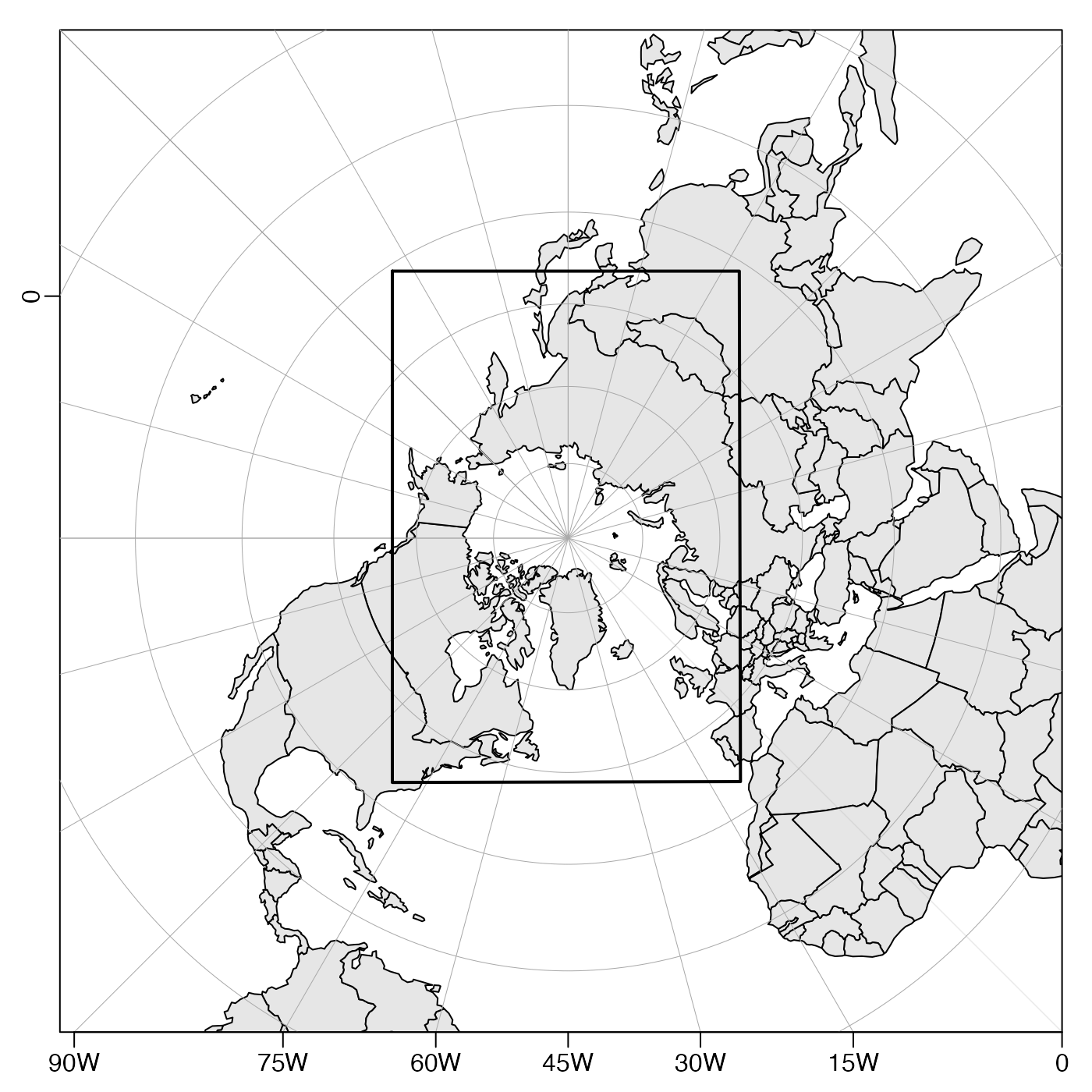
# Demonstrate a high-latitude view using a built-in "CRS" value that is used
# by the National Snow and Ice Data Center (NSIDC) for representing
# the northern-hemisphere ice zone.  The view is meant to mimic the figure
# at the top of the document entitled "A Guide to NSIDC's Polar Stereographic
# Projection" at https://nsidc.org/data/user-resources/help-center, with the
# box indicating the region of the NSIDC grid.
library(oce)
data(coastlineWorld)
projection <- sf::st_crs("EPSG:3413")
cat(projection$proj4string, "\n") # see the projection details
#> +proj=stere +lat_0=90 +lat_ts=70 +lon_0=-45 +x_0=0 +y_0=0 +datum=WGS84 +units=m +no_defs 
par(mar = c(2, 2, 1, 1)) # tighten margins
mapPlot(coastlineWorld,
    projection = projection,
    col = gray(0.9), geographical = 4,
    longitudelim = c(-180, 180), latitudelim = c(10, 90)
)
# Coordinates of box from Table 6 of the NSIDC document
box <- cbind(
    -360 + c(168.35, 102.34, 350.3, 279.26, 168.35),
    c(30.98, 31.37, 34.35, 33.92, 30.98)
)
mapLines(box[, 1], box[, 2], lwd = 2)