Compute the potential temperature of seawater, denoted \(\theta\)
in the UNESCO system, and pt in the GSW system.
Arguments
- salinity
either salinity (PSU) (in which case
temperatureandpressuremust be provided) or anoceobject (in which casesalinity, etc. are inferred from the object).- temperature
in-situ temperature (\(^\circ\)C), defined on the ITS-90 scale; see “Temperature units” in the documentation for
swRho(), and the examples below.- pressure
pressure (dbar)
- referencePressure
reference pressure (dbar)
- longitude
longitude of observation (only used if
eos="gsw"; see “Details”).- latitude
latitude of observation (only used if
eos="gsw"; see “Details”).- eos
equation of state, either
"unesco"(references 1 and 2) or"gsw"(references 3 and 4).- debug
an integer specifying whether debugging information is to be printed during the processing. This is a general parameter that is used by many
ocefunctions. Generally, settingdebug=0turns off the printing, while higher values suggest that more information be printed. If one function calls another, it usually reduces the value ofdebugfirst, so that a user can often obtain deeper debugging by specifying higherdebugvalues.
Details
Different formulae are used depending on the equation of state. If eos
is "unesco", the method of Fofonoff et al. (1983) is used
(see references 1 and 2).
Otherwise, swTheta uses gsw::gsw_pt_from_t() from
the gsw package.
If the first argument is a ctd or section object, then values
for salinity, etc., are extracted from it, and used for the calculation, and
the corresponding arguments to the present function are ignored.
References
Fofonoff, P. and R. C. Millard Jr, 1983. Algorithms for computation of fundamental properties of seawater. Unesco Technical Papers in Marine Science, 44, 53 pp
Gill, A.E., 1982. Atmosphere-ocean Dynamics, Academic Press, New York, 662 pp.
IOC, SCOR, and IAPSO (2010). The international thermodynamic equation of seawater-2010: Calculation and use of thermodynamic properties. Technical Report 56, Intergovernmental Oceanographic Commission, Manuals and Guide.
McDougall, T.J. and P.M. Barker, 2011: Getting started with TEOS-10 and the Gibbs Seawater (GSW) Oceanographic Toolbox, 28pp., SCOR/IAPSO WG127, ISBN 978-0-646-55621-5.
See also
Other functions that calculate seawater properties:
T68fromT90(),
T90fromT48(),
T90fromT68(),
computableWaterProperties(),
locationForGsw(),
swAbsoluteSalinity(),
swAlpha(),
swAlphaOverBeta(),
swBeta(),
swCSTp(),
swConservativeTemperature(),
swDepth(),
swDynamicHeight(),
swLapseRate(),
swN2(),
swPressure(),
swRho(),
swRrho(),
swSCTp(),
swSR(),
swSTrho(),
swSigma(),
swSigma0(),
swSigma1(),
swSigma2(),
swSigma3(),
swSigma4(),
swSigmaT(),
swSigmaTheta(),
swSoundAbsorption(),
swSoundSpeed(),
swSpecificHeat(),
swSpice(),
swSpiciness0(),
swSpiciness1(),
swSpiciness2(),
swSstar(),
swTFreeze(),
swTSrho(),
swThermalConductivity(),
swViscosity(),
swZ()
Examples
library(oce)
# Example 1: test value from Fofonoff et al., 1983
stopifnot(abs(36.8818748026 - swTheta(40, T90fromT68(40), 10000, 0, eos = "unesco")) < 0.0000000001)
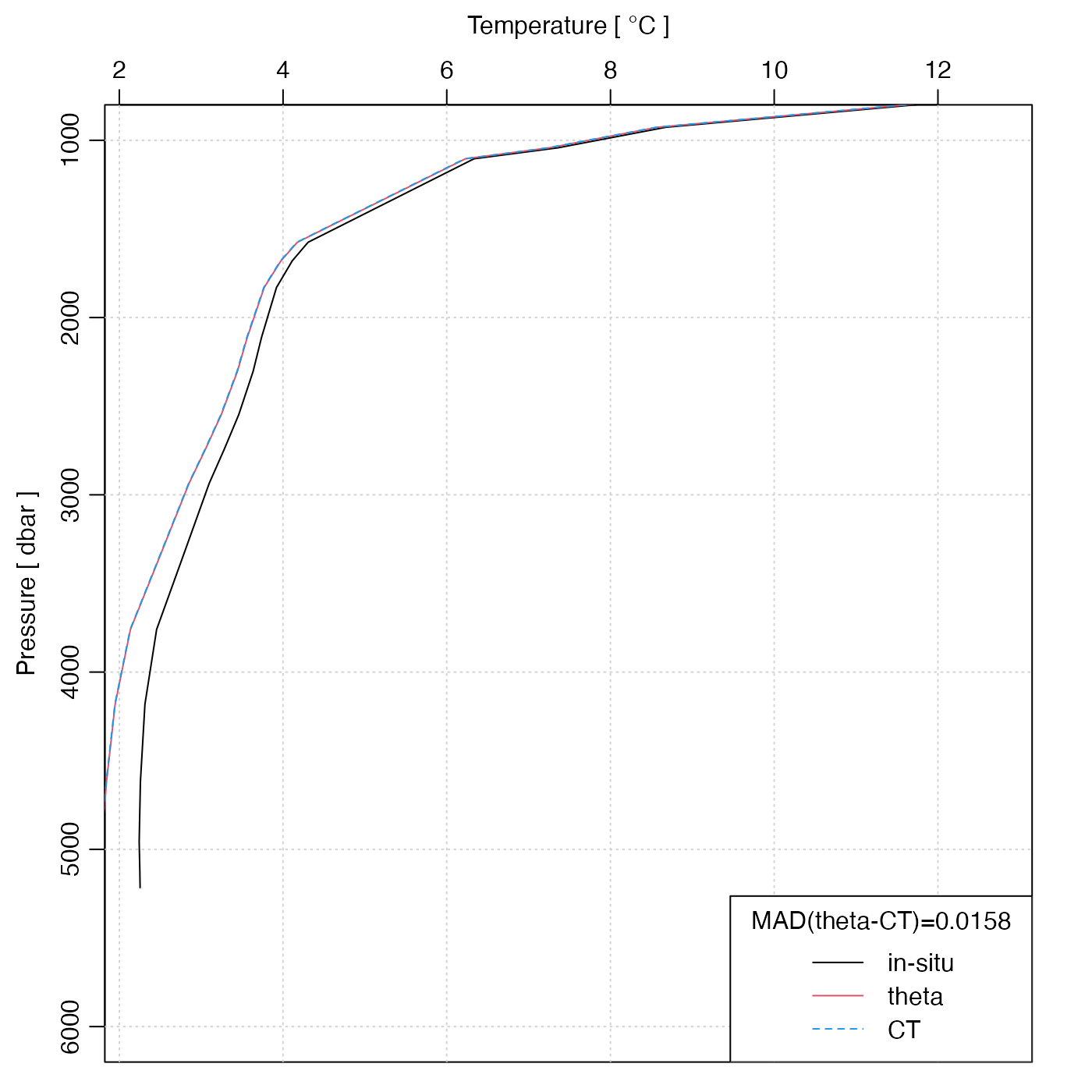
# Example 2: a deep-water station. Note that theta and CT are
# visually identical on this scale.
data(section)
stn <- section[["station", 70]]
plotProfile(stn, "temperature", ylim = c(6000, 1000))
lines(stn[["theta"]], stn[["pressure"]], col = 2)
lines(stn[["CT"]], stn[["pressure"]], col = 4, lty = 2)
legend("bottomright",
lwd = 1, col = c(1, 2, 4), lty = c(1, 1, 2),
legend = c("in-situ", "theta", "CT"),
title = sprintf("MAD(theta-CT)=%.4f", mean(abs(stn[["theta"]] - stn[["CT"]])))
)