Compute the sound absorption of seawater, in dB/m.
Usage
swSoundAbsorption(
  frequency,
  salinity,
  temperature,
  pressure,
  pH = 8,
  formulation = c("fisher-simmons", "francois-garrison", "ainslie-mccolm",
    "schulkin-marsh", "thorp-extended")
)
Arguments
- frequency
the frequency of sound, in Hz.
- salinity
either practical salinity (in which case
temperatureandpressuremust be provided) or anoceobject, in which casesalinity,temperature(in the ITS-90 scale; see next item), etc. are inferred from the object, ignoring the other parameters, if they are supplied.- temperature
in-situ temperature (\(^\circ\)C), defined on the ITS-90 scale. This scale is used by GSW-style calculation (as requested by setting
eos="gsw"), and is the value contained withinctdobjects (and probably most other objects created with data acquired in the past decade or two). Since the UNESCO-style calculation is based on IPTS-68, the temperature is converted within the present function, usingT68fromT90().- pressure
pressure (dbar)
- pH
seawater pH.
- formulation
character string indicating the formulation to use. The choices are
"fischer-simmons","francois-garrison","ainslie-mccolm","schulkin-marsh" and"thorp-extended"`. These may be abbreviated using sufficient initial letters to be distinct.
Details
Salinity and pH are ignored in this formulation. Several formulae may be found in the literature, and they give results differing by 10 percent, as shown in reference 3 for example. For this reason, it is likely that more formulations will be added to this function, and entirely possible that the default may change.
Note that the "thorp-extended" model is an extended version of Thorp's equation,
as discussed in References 8, 9 and 10. Following these citations will lead to
Thorp's original paper, which does not include the extended equation. The original
source for this extended version is not clear.
References
F. H. Fisher and V. P. Simmons, 1977. Sound absorption in sea water. Journal of the Acoustical Society of America, 62(3), 558-564.
R. E. Francois and G. R. Garrison, 1982. Sound absorption based on ocean measurements. Part II: Boric acid contribution and equation for total absorption. Journal of the Acoustical Society of America, 72(6):1879-1890.
http://resource.npl.co.uk/acoustics/techguides/seaabsorption/Michael A. Ainslie, James G. McColm; A simplified formula for viscous and chemical absorption in sea water. J. Acoust. Soc. Am. 1 March 1998; 103 (3): 1671–1672.
M. Schulkin, H. W. Marsh; Sound Absorption in Sea Water. J. Acoust. Soc. Am. 1 June 1962; 34 (6): 864–865.
H. Thorp. Analytic description of the low frequency attenuation coefficient. Journal of Acoustical Society of America, 1967.
T. Melodia, H. Kulhandjian, L.-C. Kuo, and E. Demirors, "Advances in underwater acoustic networking," Mobile Ad Hoc Networking: Cutting Edge Directions, pp. 804-852, 2013.
Al-Aboosi, Yasin & Al-Aboosi, Jenan. (2018). Study of Absorption Loss Effects on Acoustic Wave Propagation in Shallow Water Using Different Empirical Models. International Journal of Advances in Applied Sciences.
Milica Stojanovic. 2006. On the relationship between capacity and distance in an underwater acoustic communication channel. In Proceedings of the 1st International Workshop on Underwater Networks (WUWNet '06). Association for Computing Machinery.
A. Sehgal, I. Tumar and J. Schonwalder, "Variability of available capacity due to the effects of depth and temperature in the underwater acoustic communication channel," OCEANS 2009-EUROPE, Bremen, Germany, 2009.
See also
Other functions that calculate seawater properties:
T68fromT90(),
T90fromT48(),
T90fromT68(),
computableWaterProperties(),
locationForGsw(),
swAbsoluteSalinity(),
swAlpha(),
swAlphaOverBeta(),
swBeta(),
swCSTp(),
swConservativeTemperature(),
swDepth(),
swDynamicHeight(),
swLapseRate(),
swN2(),
swPressure(),
swRho(),
swRrho(),
swSCTp(),
swSR(),
swSTrho(),
swSigma(),
swSigma0(),
swSigma1(),
swSigma2(),
swSigma3(),
swSigma4(),
swSigmaT(),
swSigmaTheta(),
swSoundSpeed(),
swSpecificHeat(),
swSpice(),
swSpiciness0(),
swSpiciness1(),
swSpiciness2(),
swSstar(),
swTFreeze(),
swTSrho(),
swThermalConductivity(),
swTheta(),
swViscosity(),
swZ()
Author
Dan Kelley and João Resende. Kelley wrote an early version of
this function, which supported only the "fisher-simmons" and
"francois-garrison" formulations. The "ainslie-mccolm", schulkin-marsh" and "thorp-extended"` formulations were added in a GitHub pull request
(number 2345) submitted on 2025-09-04 by Resende, who also added a
comparison plot to the documentation.
Examples
# Fisher & Simmons (1977 table IV) gives 0.52 dB/km for 35 PSU, 5 degC, 500 atm
# (4990 dbar of water)a and 10 kHz
alpha <- swSoundAbsorption(35, 4, 4990, 10e3)
# reproduce part of Fig 8 of Francois and Garrison (1982 Fig 8)
f <- 1e3 * 10^(seq(-1, 3, 0.1)) # in Hz
plot(f / 1000, 1e3 * swSoundAbsorption(f, 35, 10, 0, formulation = "fr"),
xlab = " Freq [kHz]", ylab = " dB/km", type = "l", log = "xy"
)
lines(f / 1000, 1e3 * swSoundAbsorption(f, 0, 10, 0, formulation = "fr"), lty = "solid")
legend("topleft", lty = c("solid", "dashed"), legend = c("S=35", "S=0"))
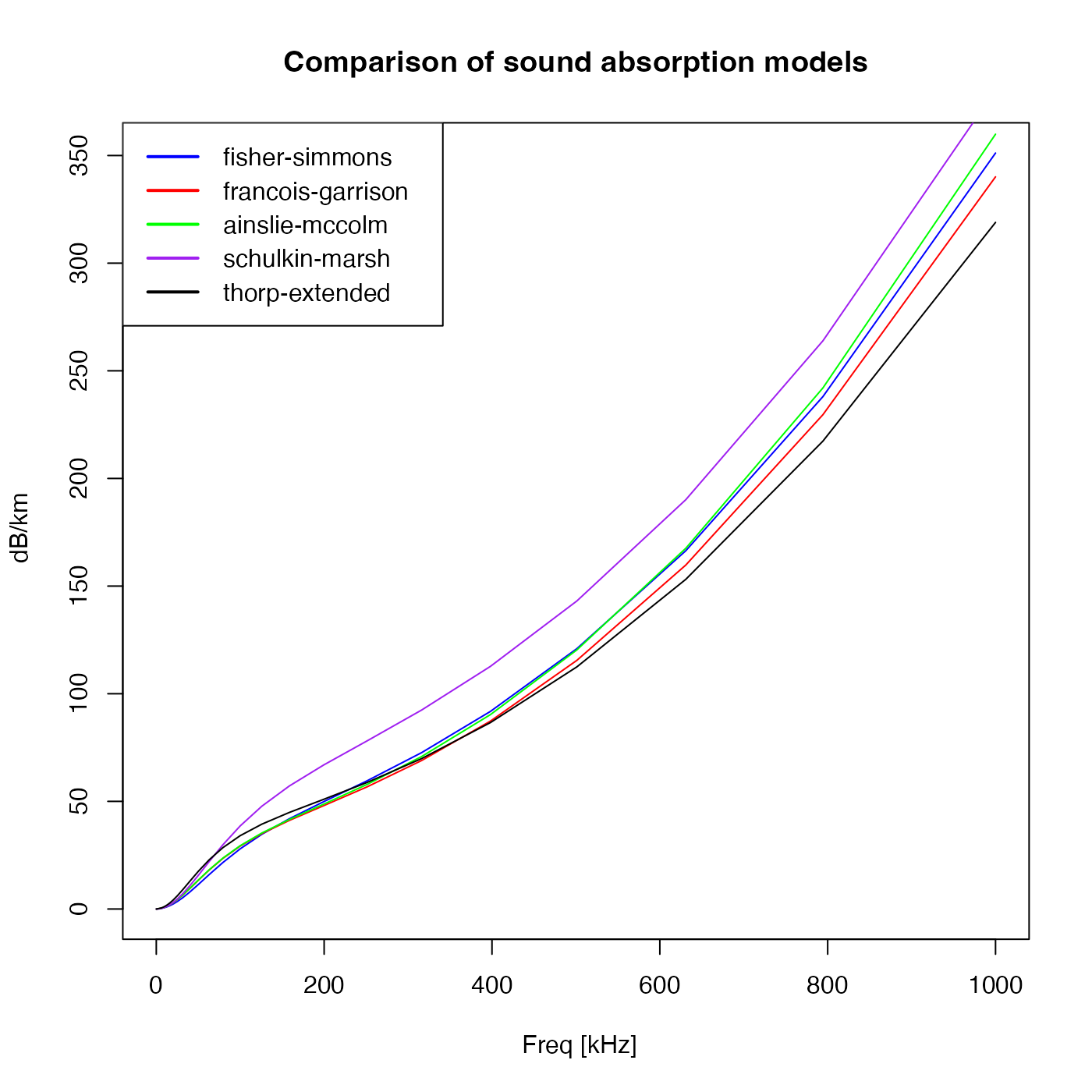
 # Comparison of the supported absorption models
f <- 1e3 * 10^(seq(-1, 3, 0.1)) # in KHz
plot(f / 1000, 1e3 * swSoundAbsorption(f, 35, 10, 1000, formulation = "fi"),
xlab = " Freq [kHz]", ylab = " dB/km", type = "l", col = "blue"
)
lines(f / 1000, 1e3 * swSoundAbsorption(f, 35, 10, 1000, formulation = "fr"), col = "red")
lines(f / 1000, 1e3 * swSoundAbsorption(f, 35, 10, 1000, formulation = "ai"), col = "green")
lines(f / 1000, 1e3 * swSoundAbsorption(f, 35, 10, 1000, formulation = "sc"), col = "purple")
lines(f / 1000, 1e3 * swSoundAbsorption(f, 35, 10, 1000, formulation = "th"), col = "black")
legend("topleft", legend = c(
"fisher-simmons", "francois-garrison",
"ainslie-mccolm", "schulkin-marsh", "thorp-extended"
), col = c("blue", "red", "green", "purple", "black"), lty = 1, lwd = 2)
title("Comparison of sound absorption models")
# Comparison of the supported absorption models
f <- 1e3 * 10^(seq(-1, 3, 0.1)) # in KHz
plot(f / 1000, 1e3 * swSoundAbsorption(f, 35, 10, 1000, formulation = "fi"),
xlab = " Freq [kHz]", ylab = " dB/km", type = "l", col = "blue"
)
lines(f / 1000, 1e3 * swSoundAbsorption(f, 35, 10, 1000, formulation = "fr"), col = "red")
lines(f / 1000, 1e3 * swSoundAbsorption(f, 35, 10, 1000, formulation = "ai"), col = "green")
lines(f / 1000, 1e3 * swSoundAbsorption(f, 35, 10, 1000, formulation = "sc"), col = "purple")
lines(f / 1000, 1e3 * swSoundAbsorption(f, 35, 10, 1000, formulation = "th"), col = "black")
legend("topleft", legend = c(
"fisher-simmons", "francois-garrison",
"ainslie-mccolm", "schulkin-marsh", "thorp-extended"
), col = c("blue", "red", "green", "purple", "black"), lty = 1, lwd = 2)
title("Comparison of sound absorption models")