Add Tissot Indicatrices to a Map

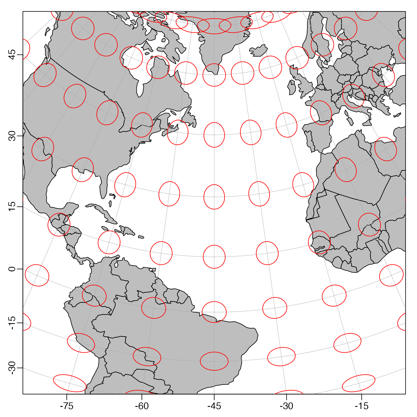
Plot ellipses at grid intersection points, as a method for indicating the distortion inherent in the projection, somewhat analogous to the scheme used in reference 1. (Each ellipse is drawn with 64 segments.)

Usage

mapTissot(grid = rep(15, 2), scale = 0.2, crosshairs = FALSE, ...)

Arguments

grid

numeric vector of length 2, specifying the increment in longitude and latitude for the grid. Indicatrices are drawn at e.g. longitudes seq(-180, 180, grid[1]).

scale

numerical scale factor for ellipses. This is multiplied by min(grid) and the result is the radius of the circle on the earth, in latitude degrees.

crosshairs

logical value indicating whether to draw constant-latitude and constant-longitude crosshairs within the ellipses. (These are drawn with 10 line segments each.) This can be helpful in cases where it is not desired to use mapGrid() to draw the longitude/latitude grid.

...

extra arguments passed to plotting functions, e.g. col="red" yields red indicatrices.

References

1. Snyder, John P., 1987. Map Projections: A Working Manual. USGS Professional Paper: 1395

See also

A map must first have been created with mapPlot().

Other functions related to maps: formatPosition(), lonlat2map(), lonlat2utm(), map2lonlat(), mapArrows(), mapAxis(), mapContour(), mapCoordinateSystem(), mapDirectionField(), mapGrid(), mapImage(), mapLines(), mapLocator(), mapLongitudeLatitudeXY(), mapPlot(), mapPoints(), mapPolygon(), mapScalebar(), mapText(), oceCRS(), oceProject(), shiftLongitude(), usrLonLat(), utm2lonlat()

Author

Dan Kelley

Examples

# \donttest{
library(oce)
data(coastlineWorld)
par(mfrow = c(1, 1), mar = c(2, 2, 1, 1))
p <- "+proj=aea +lat_1=10 +lat_2=60 +lon_0=-45"
mapPlot(coastlineWorld,
    projection = p, col = "gray",
    longitudelim = c(-90, 0), latitudelim = c(0, 50)
)
mapTissot(c(15, 15), col = "red")

# }