Test Case with Table Tennis Ball

Dan Kelley (https://orcid.org/0000-0001-7808-5911)

2024-08-06

Abstract. This vignette outlines a test of the model against theory for a very simple mooring, and ends with an idea for an instrument to measure flow based on mooring dynamics.

Introduction

As a test of the mooring code, and a possible motivation for a simple experiment, consider a table-tennis ball attached with a thin fishing line to a solid immovable object. These balls are very buoyant in water, consisting of a light and thin material with air inside. By contrast, fishing line is nearly neutrally buoyant in water. The area of the ball will appreciably exceed that of the line, unless the line is very long, and therefore the drag on the ball will be much larger than the drag on the line.

Theory

For simplicity, we may assume that the line has zero drag, and zero buoyancy.

Let $L$ be the length of the line and $R$ the radius of the ball. Let the water density be $\rho$. Assuming that the density of the ball (and air inside) is much less than water density, we may approximate the ball buoyancy force as

$$\begin{equation} \tag{1} B = \frac{4}{3}\pi \rho g R^3 \end{equation}$$

where $g$ is the acceleration due to gravity. The drag on the ball may be approximated as

$$\begin{equation} \tag{2} D = \frac{1}{2} C_D \rho \pi R^2 u^2 \end{equation}$$

where $C_D$ is a drag coefficient and $u$ is the water speed in the $x$ direction.

We assume a steady state. If $\tau$ represents tension in the fishing line, and $\phi$ the angle the line makes to the vertical, then force balance in the horizontal and vertical directions requires that

$$\begin{equation} \tag{3} \tau\sin\phi = D \end{equation}$$

and

$$\begin{equation} \tag{4} \tau\cos\phi = B \end{equation}$$ respectively. Dividing these yields $$\begin{equation} \tag{5} \phi = \tan^{-1}\frac{D}{B} \end{equation}$$

From the above, it follows that tension in the line is

$$\begin{equation} \tag{6} \tau = \frac{B}{\cos\phi} \end{equation}$$

that the ball is at position

$$\begin{equation} \tag{7} x' = L\sin\phi \end{equation}$$

and that it is at height

$$\begin{equation} \tag{8} z' = L - L\cos\phi \end{equation}$$

above the bottom.

It is easy to imagine an experimental setup in which $x'$ might be measured (replace the anchor with a rod held vertical in the water column, with the line attached at the bottom, and sight downwards to get the distance of the float from the rod).

Test

The predictions can be tested against the knockdown() function as follows. This imagines a river of depth 0.5m (about knee-deep) and a 1m/s current (about walking speed). Note that the prediction of the mooring code matches that (circled in blue) of the formulae given above.

library(testthat)
L <- 0.5 # tank depth, m
diameter <- 0.04 # ping-pong balls have 40mm diameter
R <- diameter / 2
area <- pi * R^2
volume <- 4 / 3 * pi * R^3
rho <- 1027
deltaRho <- rho # water vs air (round numbers)
g <- 9.81
B <- g * deltaRho * volume # buoyancy force [N]
CD <- 1
u <- 0.5 # speed, m/s
D <- 0.5 * CD * area * rho * u^2 # ddrag force [N]
phi <- atan2(D, B)
x <- L * sin(phi)
l <- L * cos(phi)
tau <- B / cos(phi)

library(mooring)

## Loading required package: S7

f <- float("pingpong", B / g, height = 0, area = pi * R^2, CD = 1)
expect_equal(B / g, buoyancy(f))
expect_equal(D, drag(f, u = u))

w <- wire("gossamer", length = L, buoyancyPerMeter = 0, areaPerMeter = 0, CD = 0)
a <- anchor("fake", buoyancy = -1000, height = 0, CD = 0)
m <- mooring(a, w, f, waterDepth = L)

ms <- segmentize(m, L / 10)
msk <- knockdown(ms, u = u)
plot(msk, fancy = TRUE)
# Check against theory
points(x, L - l, col = 2, cex = 2)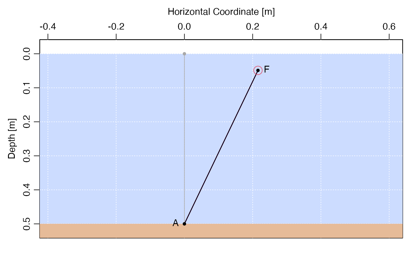

Test of package against direct computation. The black dot is the float position computed in the package, whereas the red circle is the result of direct computation using equations 7 and 8.

Results

The theory and the calculations using knockdown() agree well. There are three main observables that might be part of an experiment to test this in a natural environment.

1. The horizontal shift of the float, $x'$. Here, a $0.5$ m/s current is predicted to yield $x'=21.6$ cm.
2. The vertical float displacement over the zero-velocity case, $z'$. Here, the prediction is $4.9$ cm.
3. The tension in the line, $\tau$, is predicted to be $`r round(tau,3)`$ Newtons, so that an anchor would need to have mass exceeding 38.1 g to avoid lifting by the drag. This mass rises to 74.3 g in a 1 m/s current, which is slightly less than the mass of a 3/4-inch bolt, 136 g, and well under the weight of a 1-inch bolt, 195 g. This suggests that a 1-inch bolt might be a good anchor for a demonstration of this effect in a flume. (See https://www.portlandbolt.com/products/nuts/hex-nuts/ for a table of bolt properties.)

Measuring currents

Any of $x'$, $z'$ and $\tau$ could be measured in a classroom or laboratory setting, but measuring tension might be harder in a field test, and so a field apparatus should focus on measuring $x'$ and $x'$. This would not be difficult, for this range of current, using a metre-stick, to which is attached a table-tennis ball with 1 m of thin mono-filament fishing line. A value of $z'$ could be obtained by lowering the rod slowly, until the float just sinks below the surface, and observing water level on the stick’s distance markings. A value of $x'$ could be obtained with a second meter stick held horizontally so that the ball position could be observed from overhead.

In a laboratory setting, or with a bit of engineering for a field setting, the tension could be measured. An advantage of that method would be that it could be digitized and, using a microcontroller to do the calculations shown here, a readout could show the current speed.