Mooring Model

Dan Kelley (https://orcid.org/0000-0001-7808-5911)

2024-08-06

Introduction

Anchored oceanographic mooring lines are deformed by currents, in much the same way as trees are bent by wind. For very simple moorings, e.g. consisting of a single float connected by a uniform cable to an anchor at the bottom, the deformation can be calculated if the current is uniform. The physics is analogous to the sagging of telephone lines between poles, and falls into the general category of a catenary. However, things are more complicated for depth-varying currents, and for mooring lines that consist of many elements, of varying buoyancy and drag, connected by wires, chains, etc., that are also of varying buoyancy and drag.

An approach to analysing realistic oceanographic moorings is to use lumped-mass theory, in which elements such as floats and instrument packages are parameterized by their buoyancy and drag characteristics, and in which cables envisioned as connected line elements. This approach was taken by Moller (1976) in a Fortran program, and more recently by Dewey (1999) in a GUI-based Matlab system. The present treatment is of similar foundation, although with some added simplifications (such as unidirectional current) that are relevant to the basic problem of computing “knock-down”, i.e. the vertical displacement of instruments that is caused by slanting of the mooring line.

Model

Consider the case of unidirectional horizontal current aligned with the $x$ axis. Following oceanographic convention, let $z$ be the vertical coordinate, positive upwards, with $z=0$ at the surface. The mooring is modelled as a series of $n$ connected elements, with the top element being numbered $i=1$ and the bottom one numbered $i=n$.

Water density and velocity are assumed to be a functions of depth, with values $\rho_i$ and $u_i$ at the location $z_i$ of the $i$-th element.

Each element is described by the following properties.

• Height, $H_i$ [m]. This is is the vertical extent of the element as placed in a completely taut (i.e. vertical) mooring.
• Area, $A_i$ [m$^2$] projected in the $x$ direction, again for an element as it would be oriented in a taut mooring.
• Buoyancy ‘force’ expressed in kilograms, i.e. the actual force in Newtons, divided by $g$, the acceleration due to gravity. For a solid object such as a float or instrument, this is a simple number, denoted $m_i$ below. For a wire or chain, it is expressed per unit length of cable, i.e. in kg/m, and denoted $\mu_i$ below. Manufacturers tend to provide $m$ or $\mu$ values in technical documentation about mooring components. Note that they refer to in-water buoyancy force, but the distinction between freshwater and seawater is seldom made clear.
• Drag coefficient, $C_i$, defined as the ratio of drag force, $D_i$, to $\frac{1}{2}A_i\rho_i u_i|u_i|$.

Figure 1. Force diagram, showing an idealization of a table-tennis ball at the end of a very thin 0.5m fishing line in a 1 m/s current flowing in a river that is 0.5m deep. Arrows show forces in the $i$-th element (with $i=1$ in this case), and the corresponding angle is indicated alongside the gray line that represents the stagnant case. The brown region is the sediment below the river, and the dot is an anchor (element $i=2$, for which there is no force calculation since it assumed to be immobile).

A tension force exists between each interior mooring element. The tension below the $i$-th interior element (thus pulling downward on it) is denoted $T_i$. This is defined for all elements of a mooring except for the bottom one, which is labelled $i=n$.

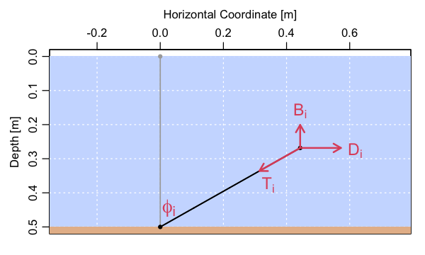
The tension force is directed vertically if there is no current, but acquires a horizontal component if there is a current, because drag from the current will distort the mooring shape. The angle made by the $i$-th element to the vertical is represented with $\phi_i$. Determining these two quantities, $T$ and $\phi$, is the key to inferring the response of a mooring to currents.

Quasi-steady dynamics are assumed, so that forces must balance in both the horizontal and vertical directions. The tension force has components in both the $x$ and $z$ directions, but the buoyancy force (defined as positive for objects that would rise if unattached to a mooring) acts only in the vertical, upwards if $m$ or $\mu$ is positive.

The buoyancy force for a solid object such as an anchor or a float is found with $$\begin{equation} \tag{1} B_i = -g m_i \end{equation}$$ while it is represented with $$\begin{equation} \tag{2} B_i = -g \mu_i \Delta l_i \end{equation}$$ for a portion of a cable of length $\Delta l_i$.

The drag force is expressed with $$\begin{equation} \tag{3} D_i = \frac{1}{2} A_i C_i \rho_i u_i |u_i| \end{equation}$$ where $A_i$ is the area projected in the flow direction.

With these definitions, a steady-state assumption dictates that forces must be balanced in the horizontal and vertical directions for each element of the mooring.

Consider the case of a mooring consisting of $n$ elements attached to an immovable bottom anchor, and let the index $i=1$ refer to the top element, with $i$ increasing to $i=n$ at the anchor.

Three forces are involved in this situation: (a) a horizontal drag force, $D$, associated with the current, (b) a vertical buoyancy force, $B$, caused by a density mismatch between a component and the background water, and (c) a tension force, $\tau$, along the connection between elements. The tension force has only a vertical component for an upright mooring, but horizontal components occur for a mooring that is tilted by a current.

By definition, the top element has no tension from above, and so a consideration of its force balance yields $$\begin{equation} \tag{4} D_1 = \tau_1 \sin\phi_1 \end{equation}$$ along with $$\begin{equation} \tag{5} B_1 = \tau_1 \cos\phi_1 \end{equation}$$ where $\tau_1$ is the tension between this element and the one below it, and $\phi_1$ is the angle that this tension force makes to the vertical.

Consider first the case of a depth-independent current, so that the drag $D_i$ on the $i$-th element may be computed without consideration for the position of the element in the water column. In such a case, both $D_1$ and $B_1$ are known, these two equations may be solved for $\tau_1$ and $\phi_1$, yielding $$\begin{equation} \tag{6} \tau_1 = \sqrt{D_1^2 + B_1^2} \end{equation}$$ and $$\begin{equation} \tag{7} \phi_1 = \tan^{-1}\frac{D_1}{B_1} \end{equation}$$

In the case of a single anchor, a short wire, and a single float, equations 6 and 7 will yield a solution for the angle of the wire, which in turn yields a value for the depth of that float. Now, we may relax the assumption of depth-independent current, by a simple scheme: solve the equations again with the updated float depth, in which case the drag will be altered from the value initially inferred. This process can then be repeated, yielding a more accurate estimate of the float depth and thus of the drag. Iterating this process can thus yield a practical estimate of the configuration of this simple mooring.

If there are more than 2 elements in the mooring, a similar line of reasoning may be extended to the next element, although now there is a tension force pulling upward. This situation is described by $$\begin{equation} \tag{8} D_2 + \tau_1 \sin\phi_1 = \tau_2 \sin\phi_2 \end{equation}$$ and $$\begin{equation} \tag{9} B_2 + \tau_1 \cos\phi_1 = \tau_2 \cos\phi_2 \end{equation}$$

Since $\phi_1$ and $\tau_1$ are known from Equation 5, Equation 6 may be solved for $\tau_2$ and $\phi_2$, using $$\begin{equation} \tag{10} \tau_2 = \sqrt{(D_2+\tau_1\sin\phi_1)^2 + (B_2+\tau_1\cos\phi_1)^2} \end{equation}$$ and $$\begin{equation} \tag{11} \phi_2 = \tan^{-1}\frac{D_2+\tau_1\sin\phi_1}{B_2+\tau_1\cos\phi_1} \end{equation}$$

This may be generalized to larger moorings, with $$\begin{equation} \tag{12} \tau_i = \sqrt{(D_i+\tau_{i-1}\sin\phi_{i-1})^2+(B_i+\tau_{i-1}\cos\phi_{i-1})^2} \end{equation}$$ and $$\begin{equation} \tag{13} \phi_i = \tan^{-1}\frac{D_i+\tau_{i-1}\sin\phi_{i-1}}{B_i+\tau_{i-1}\cos\phi_{i-1}} \end{equation}$$ applying for elements $i=2,\dots,n-1$. The limit ends at $n-1$ because is no tension below the bottom element, so neither $\tau_n$ nor $\phi_n$ can be defined.

This leads to a simple way to describe mooring response to a depth-independent current, in which $D_i$ and $B_i$ are known quantities for each $i$ from 1 to $n$:

1. First, use Equations 4 through 7 to compute $\tau_1$ and $\phi_1$, the angle and tension below the top ($i=1)$ element.
2. Use Equations 12 and 13 to compute $\tau_i$ and $\phi_i$ for $i=2$.
3. Continue as in step 2, until reaching the bottom ($i=n-1$) element.
4. Update the depth location of all elements and repeat the computation of steps 1 to 3. Repeat this procedure until some convergence criterion is reached; Moller (1976) suggested basing this criterion on the changes in $\phi$ from one iteration to the next.

Example

Figure 2 shows the result of simulating a 20-inch Hydro Float Mooring Buoy (with $34.5$kg buoyancy) connected to a bottom anchor with 100 m of quarter-inch jacketed wire (with $-13$kg/m of buoyancy), in a depth-independent 0.5 m/s (roughly 1 knot) current. Note that the float is predicted to sink $7.7$m with this current. However, the predicted knockdown increases to $41.2$m with a $1$m/s current, suggesting that this float would be of limited utility in supporting an oceanographic mooring a region with strong currents.

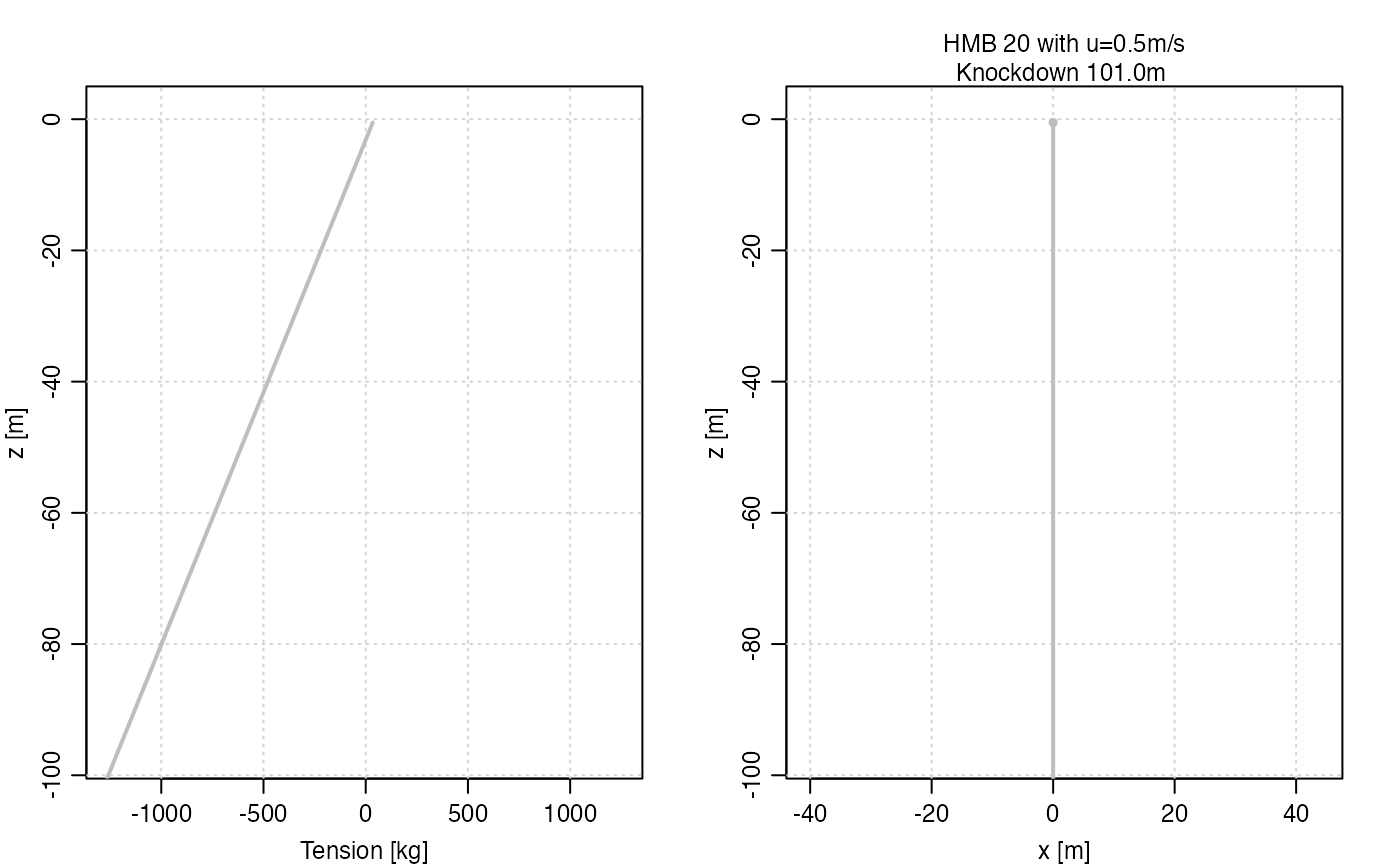
Figure 2. Response of a mooring to a $u=1$m/s current, as described in the text. Left: Cable tension, in kg, with gray for the $u=0$ case and black for the $u=1$m/s case. Right: Mooring shape, with same colour scheme as left panel.

Special case: negligible currents

As a special case, if $u_i=0$ for all $i$, then there will be no drag, and so (assuming adequate buoyancy), the mooring will be aligned in the vertical, and the vertical equation becomes $$\begin{equation} \tag{14} \tau_{i+1} = \tau_i + B_i \end{equation}$$ which yields $$\begin{equation} \tag{15} \tau_i = \sum_{j=1}^{i-1} B_j \end{equation}$$ for $i>1$. Physically, this means that the downward tension at any level balances the total upward buoyancy force of all the elements above it. The bottom tension, $\tau_n$, may be interpreted as the minimum anchor weight that will hold the mooring in place in the absence of currents. However, it should be obvious that heavier weights will be required for practical situations.

References

Dewey, Richard K. 1999. “Mooring Design & Dynamics—a Matlab® Package for Designing and Analyzing Oceanographic Moorings.” Marine Models 1 (1): 103–57. https://doi.org/10.1016/S1369-9350(00)00002-X.

Moller, Donald A. 1976. “A Computer Program for the Design and Static Analysis of Single-Point Subsurface Mooring Systems: NOYFB.” WHOI-76-59. Woods Hole, MA: Woods Hole Oceanographic Institution. https://darchive.mblwhoilibrary.org/server/api/core/bitstreams/0f41541c-7db6-5641-8412-02f68276b439/content .