The mooring package
Dan Kelley (https://orcid.org/0000-0001-7808-5911)
2025-07-25
Source:vignettes/mooring.Rmd
mooring.RmdIntroduction
The mooring package deals with oceanographic moorings
and their deformation by horizontal currents. The theory for that
deformation is laid out in the vignetted entitled Mooring Response
to Unidirectional Flow, while the present vignette deals with using
the package.
Mooring Construction
Moorings are constructed with mooring(), the arguments
of which, called
’elementalobjects, are created byanchor(),chain(),float(),instrument(),release(), orwire()`.
These are specified from bottom to top. For example, consider a mooring
in water of depth 200m, with a 150-m long wire connecting a bottom
anchor to a float. This could be created with
## Loading required package: S7where each of the function calls that construct the arguments has
taken on a default value. To learn the possible values for any of these,
supply a first argument as the string "?", e.g. the
possible wire types (which include non-metallic wires) is:
wire("?")## [1] "1 Nylon"
## [2] "1/2 Dyneema"
## [3] "1/2in AmSteel-Blue"
## [4] "1/2in Dacron"
## [5] "1/2in Kevlar"
## [6] "1/2in Neutral Wire"
## [7] "1/2in VLS"
## [8] "1/2in wire/jack"
## [9] "1/4-1/2 WarpSpd"
## [10] "1/4in AmSteel-Blue"
## [11] "1/4in galvanized wire coated to 5/16in"
## [12] "1/4in Kevlar"
## [13] "1/4in wire rope"
## [14] "1/4in wire/jack"
## [15] "11mm Perlon"
## [16] "1in Neutral Wire"
## [17] "3/16in galvanized wire coated to 1/4in"
## [18] "3/16in wire rope"
## [19] "3/4in Dacron"
## [20] "3/4in Nylon"
## [21] "3/4in Polyprop"
## [22] "3/8in AmSteel-Blue"
## [23] "3/8in Kevlar"
## [24] "3/8in leaded polypropylene"
## [25] "3/8in wire rope"
## [26] "3/8in wire/jack"
## [27] "5/16in Kevlar"
## [28] "5/16in wire rope"
## [29] "5/16in wire/jack"
## [30] "5/8in AmSteel-Blue"
## [31] "5/8in Kevlar"
## [32] "5/8in Nylon"
## [33] "7/16in Dacron"
## [34] "7/16in Kevlar"
## [35] "7/16in VLS"
## [36] "9/16in Dacron"
## [37] "9/16in Kevlar"
## [38] "BPS Cable"
## [39] "BPS Power/Coms"More details on the functions are provided with
e.g. ?wire. Details of the objects are provided in the
vignette called Default Values for Mooring Elements. Each
element has information that the package can use to find forces that
control mooring shape. The horizontal drag force at a given water speed
depends on the object’s frontal area and drag coefficient. The vertical
buoyancy force depends on the buoyancy of the element, which is
expressed (in kg) mass equivalents (assuming
m/s
for the acceleration of gravity) for discrete elements such as floats
and instruments, and in buoyancy per length (in kg/m) for wires.
Note that new types of wire, float, etc. can be created easily, by supplying a name that is not matched in the list of built-in values. The help pages for the various functions explain what must be specified.
Actual moorings are likely to have multiple instruments, along with multiple buoyancy elements, but the mooring just created is sufficient to continue the discussion here.
Exercise 1: Produce a table of float name and buoyancy.
Exercise 2: Plot float drag vs buoyancy, and compare with expectations.
Knockdown Computation
The knockdown() function is used to compute the shape of
a mooring that is deformed by a horizontal current. It takes just two
arguments: the mooring, and the velocity. The latter may be a fixed
value (in m/s), or a function that gives velocity as a function of depth
below the water surface.
But, before applying knockdown(), it is important to
first subdivide any wire elements into smaller lengths, so
that knockdown() can compute the shape more precisely. This
is done with the segmentize() function. The following shows
how to do this with the mooring just created.
ms <- segmentize(m) # breaks wire portions into approx. 1-m segmentsand the knocked-down mooring is found with e.g.
msk <- knockdown(ms, u = 1)for a 1 m/s current.
The functions x() and z() find the
and
locations of mooring elements. Note that
at the surface and negative in the water column; use
depth() to get depth below the surface.
For example, the shape of the knocked-over mooring from the previous code block could be plotted with

Mooring shape (not to scale).
Similarly, the tension between elements is found with
tension(), and the angle that elements make to the vertical
is found with angle().
Plotting
The plot shown above is quite primitive, so the package offers a
plot() function. For example, this gives a view of tension
and shape.
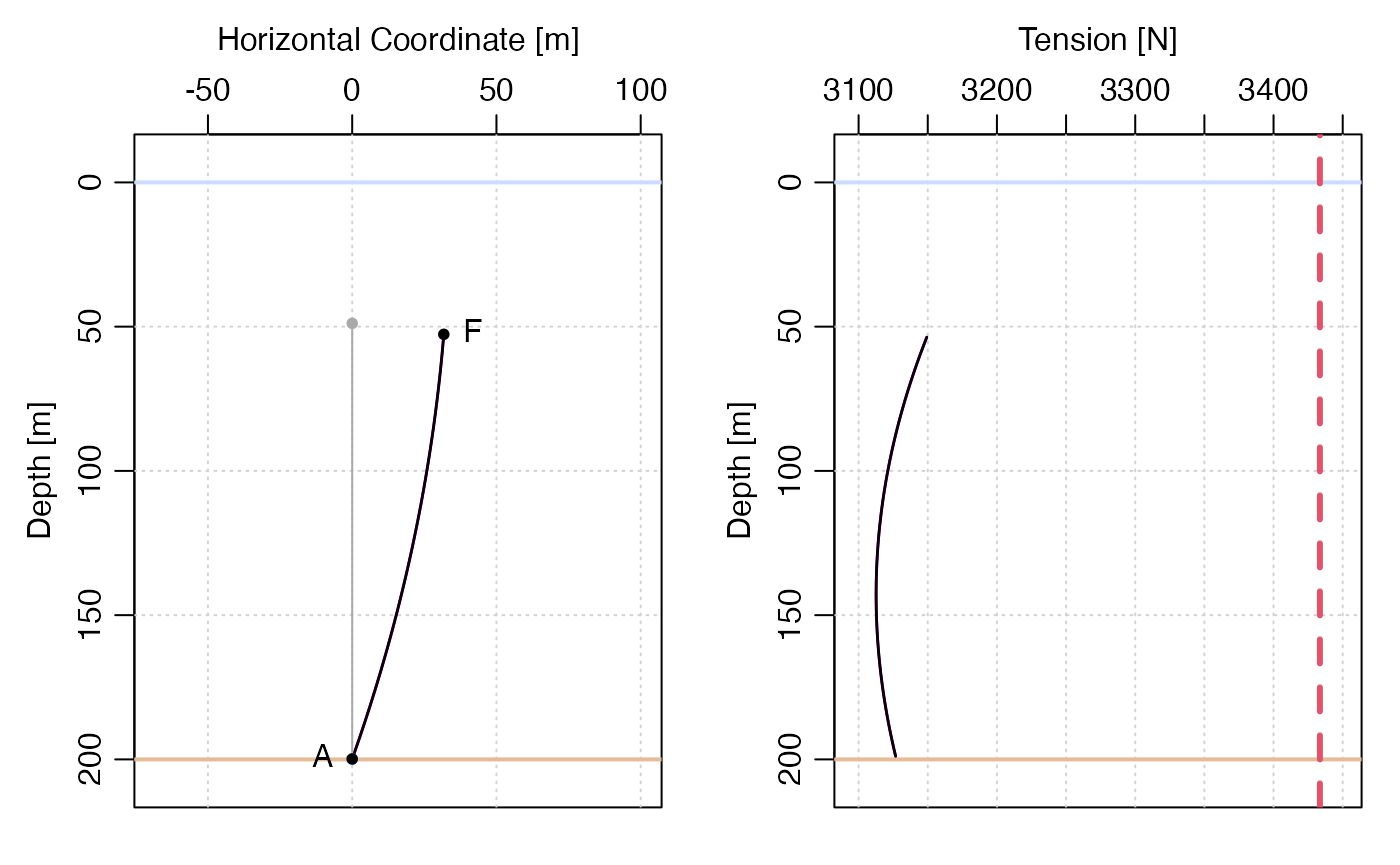
Mooring shape and tension profiles created with plot(). The red dashed line on the right-hand panel represents the anchor weight.
In both instances, the gray line is the shape that would occur with no current. Note that the shape plot uses a 1:1 aspect ratio, making it easier to understand the result. Also, note that depth is plotted here, as opposed to the shown above.
A fancier version is obtained with
par(mfrow = c(1, 2))
plot(msk, which = "shape", fancy = TRUE)
plot(msk, which = "tension", fancy = TRUE)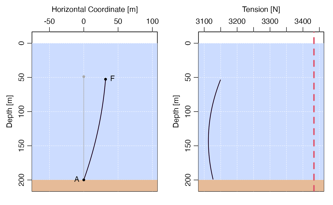
Mooring shape and tension, with water coloured blue and bottom coloured brown.
Interactive Apps
The package supplies interactive (shiny) apps, which are designed to help become familiar with the package.
-
app1(), works with moorings consisting of an anchor, a wire, and a float. -
app2(), adds an instrument, which can be placed between anchor and float. -
app2bs()is a trial version of a new aesthetic display ofapp2().
Each of these apps has controls for adjusting the simulation. Importantly, each also has a button labelled ‘Code’, which opens a pop-up window showing R code that can reproduce the plots. This can be useful for building intuition about how knockdown depends on the choice of float, wire and instrument, and also how the positions of the elements affects the deformation of the mooring in current.
The following is a screenshot of app2bs() in action.
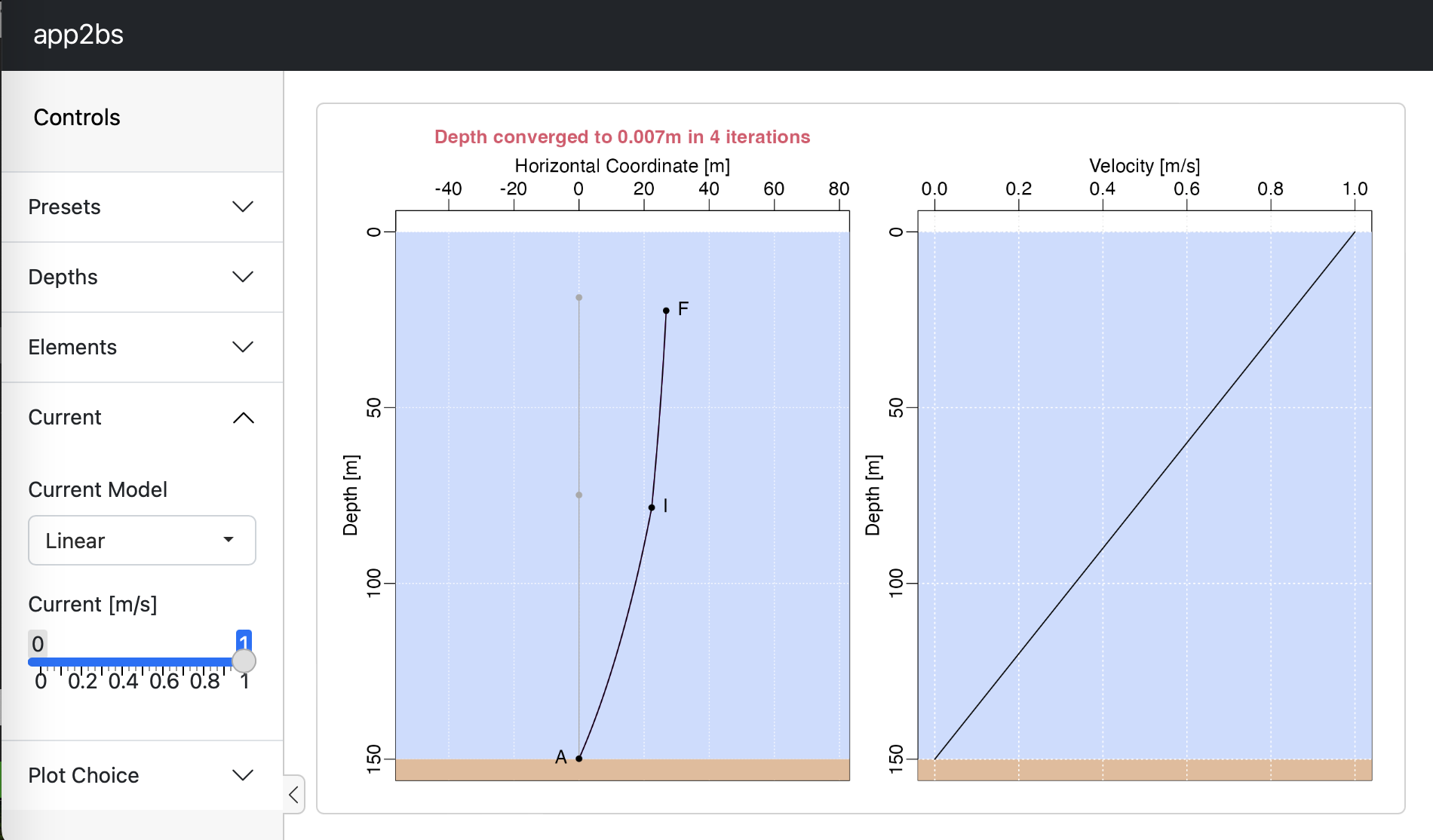
View of the app2bs() shiny application, with the ‘Current’ controller open, after increasing the value from its default of 0.5 m/s to 1 m/s.
Advanced Usage
Creating New Elements
If the first argument to an element-forming function such as
float(), instrument(), wire(),
instrument(), etc., is not in the list of built-in types,
then a new object is created. In this situation, all of the other
arguments to the function must be supplied, and it should be born in
mind that those arguments vary from type to type. For example,
i <- instrument("myNewInstrument", buoyancy = -5, height = 1, area = 0.1, CD = 1)creates a new instrument object for something that has buoyancy -5kg (meaning it weighs 5kg in seawater), height 1m, area 0.1 square metre, and drag coefficient equal to 1.
Altering Existing Elements
Strumming of wires in currents can increase wire drag coefficient by perhaps a factor of 2 (Hamilton, Fowler, and Belliveau 1997; Hamilton 1989), and simple way to account for that might be to use
w <- wire(length = 100) # default wire type
w2 <- w
w2@CD <- 2 * w2@CD
As a check, we may confirm that this doubles the drag for, say, a 1m/s current:
## [1] 534.04 1068.08All object types store a value for CD, but the other
entries depend on the type. The simplest way to find out what is stored
in a given type is to create a sample object and study it, e.g. with
float()## <mooring::floatS7>
## @ model : chr "Kiel SFS40in"
## @ buoyancy : num 320
## @ height : num 1
## @ area : num 0.785
## @ CD : num 0.65
## @ source : chr "Dewey"
## @ originalName: chr "Kiel SFS40in"
## @ x : num 0
## @ x0 : num 0
## @ z : num 0
## @ z0 : num 0
## @ phi : num 0
## @ tau : num 0
## @ group : num 0Mooring Design
A prime question in the design of a mooring is the amount of buoyancy
that will be required to maintain an essentially upright position,
despite the tendency of currents to knock it over. The
mooring package can offer guidance in this task.
As a simplified example, imagine that a mooring is to be placed in 100 m of water, with a 1/4-inch jacketed wire cable connecting a subsurface float to a bottom anchor. How will knockdown vary with current strength? To answer this, we might construct a graph as follows. Similar graphs could be done with different float and wire types.
library(mooring)
a <- anchor()
w <- wire(length = 90)
f <- float()
m <- mooring(a, w, f, waterDepth = 100)
us <- seq(0, 1.0, length.out = 10)
ms <- segmentize(m)
depths <- sapply(us, \(u) {
    msk <- knockdown(ms, u)
    depth(msk)[1]
})
par(mar = c(3, 3, 1, 1), mgp = c(2, 0.7, 0))
plot(us, depths,
    xaxs = "i", ylim = rev(range(depths)), type = "l", lwd = 2,
    xlab = "Horiz. velo. [m/s]", ylab = "Float depth [m]"
)
grid()
abline(h = 1.1 * depth(ms)[1], lty = 2)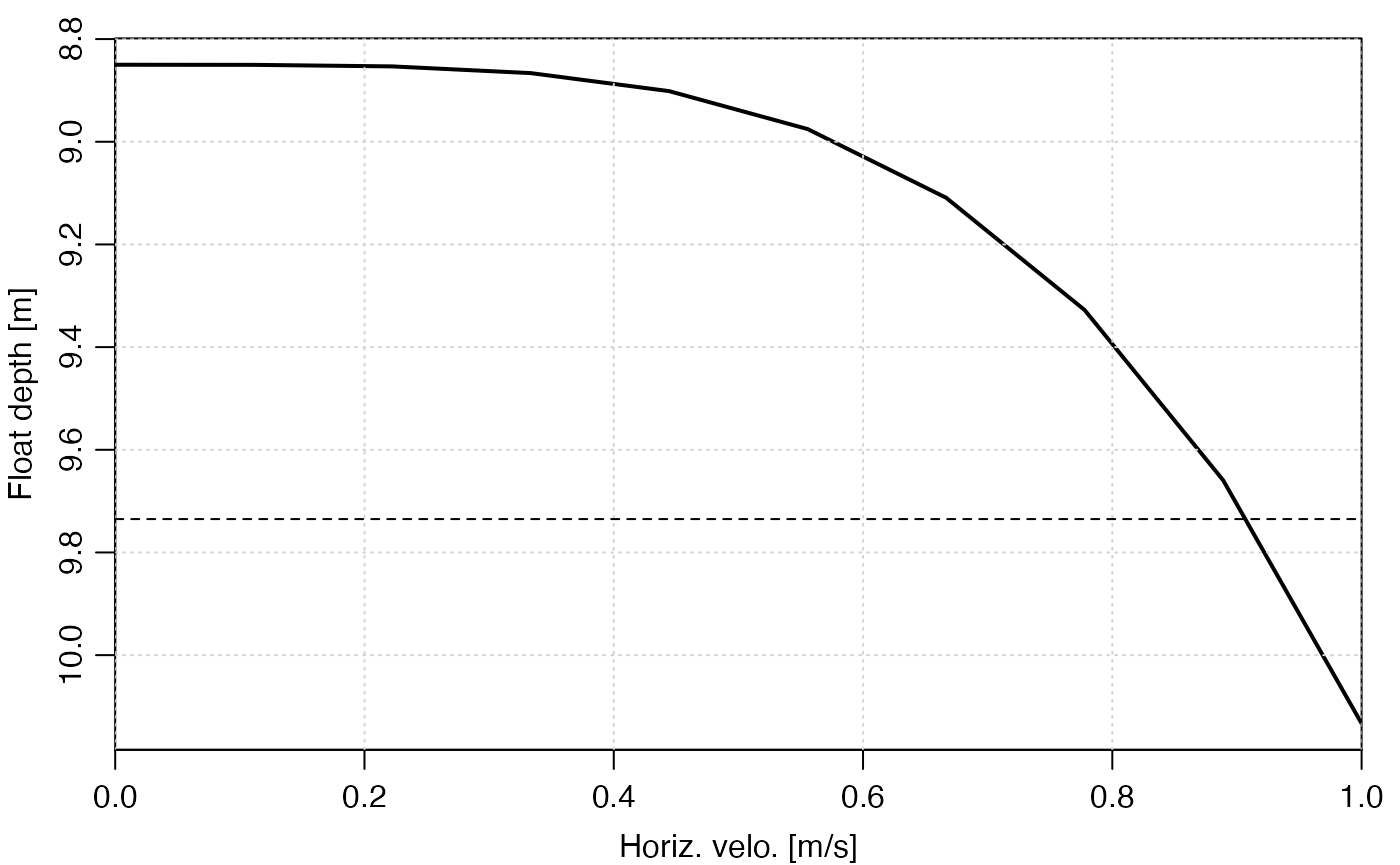
Dependence of knockdown on current. Solid: depth of top mooring element (a float). Dashed: 10% increase in that depth.
This analysis suggests that a m/s current could yield a 10 percent increase in depth of the top mooring element, so the mooring needs more buoyancy if greater mooring stiffness is required, or if currents exceed this value.
Exercise 3: Suggest a float that will hold this mooring taut in 2m/s current.
Solutions to Exercises
Exercise 1
A table of float name and buoyancy is produced with
f <- float("?") # get list of floats
b <- unlist(lapply(f, \(x) buoyancy(float(x))))
df <- data.frame(float = f, buoyancy = b)
and the 4 least-buoyancy entries are
o <- order(df$b)
df[o[1:4], ]
## float buoyancy
## 49 Top of Tow Rope 0.010
## 14 8in centre hole tfloat 2.752
## 1 11in centre hole tfloat 7.770
## 19 Billings 12in 10.000(Note that not all entries in this table are subsurface floats!)
Exercise 2
We do this in three steps (see comments in the code).
- Create a data frame of floats with non-zero buoyancy and non-zero drag. (The latter occurs for some floats that have insufficient information for the drag computation.)
- Display on a log-log plot, with buoyancy, which is reported in kg, being converted to Newtons by multiplying by m/s.
- Assuming that floats have similar constitution, and spherical shape, then buoyancy should scale as the cube of radius and drag to the square of radius. On this log-log plot, therefore, the data ought to lie along a line of slope 2/3.
# 1
library(mooring)
f <- float("?")
b <- 9.8 * unlist(lapply(f, \(x) buoyancy(float(x)))) # mult. by g to get Newtons
d <- unlist(lapply(f, \(x) drag(float(x), 1)))
ok <- b > 0 & d > 0
df <- data.frame(float = f[ok], drag = d[ok], buoyancy = b[ok])
# 2
plot(df$drag, df$buoyancy, xlab = "Drag Force [N]", ylab = "Buoyancy Force [N]", log = "xy")
# 3
drag <- seq(min(df$drag), max(df$drag), length.out = 100)
buoyancy <- drag^(3 / 2) # the factor is just for illustration
lines(drag, buoyancy)
Float drag-buoyancy relationship, in log-log scaling. Circles: data for the built-in float types, assuming a 1m/s current. Line: a scaling line of slope 3/2, with an arbitrary vertical shift for comparison with the slope of the data cloud.
The data cloud slope is similar to that of the indicated scaling line, created by assuming that drag is proportional to scale squared, while buoyancy is proportional to scale cubed. (Other factors are involved, so only the slope is of significance here.)
Much can be learned from computations of this sort. For example, it reveals why large floats are better at producing taut moorings: the buoyancy force is proportional to a higher power of scale than is the drag force. It also explains why advanced floats are designed to have lower drag coefficients, but that is another matter!
Exercise 3
To find a float that will hold this mooring reasonably taut in 2m/s
current, one approach is to use app(), which has a pulldown
menu for the float type. Another approach is to start with the table
produced in Exercise 1, and try different float models in the code given
in the “Mooring Design” section. Of course, a criterion on tautness must
be the starting point in such an analysis, and for simplicity, we take
it to be 10 percent increase in the depth of the top mooring
element.
Exploration along these lines reveals that
f <- float("CDMS 2m sphere")will suffice, as its buoyancy, 2470 kg, sufficiently exceeds the 320 kg of the default float.