A Practical Example
Dan Kelley (https://orcid.org/0000-0001-7808-5911)
2025-07-25
Source:vignettes/example.Rmd
example.RmdIntroduction
This vignette explains how to use the mooring package to
create a simulation of mooring 1840 on the Sackville Spur, based on a
diagram that appeared in a report provided by the Bedford Institute of
Oceanography (Department of Fisheries and Oceans, Canada) containing a
Notice to Mariners document.
Source Document
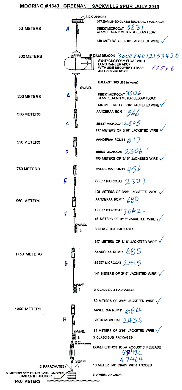
Figure 1. Diagram for Bedford Institute of Oceanograph mooring 1840 on Sackville Spur
Mooring Construction
## Loading required package: S7
# Abbreviations for convenience
W <- function(length) wire("3/16in galvanized wire coated to 1/4in", length = length)
BUB3 <- float("streamlined BUB 3 Viny balls")
RCM11 <- instrument("RCM-11 in frame") # "AANDERAA RCM11"
microcat <- instrument("SBE37 microcat clamp-on style") # "SBE MICROCAT"

# The database does not have a 5-wheel anchor, but we may construct
# one as follows.  Note that this does not matter to the knockdown
# calculation, but it might be useful in cases where an anchor was
# not heavy enough to hold the mooring in place.
buoyancy <- 5 / 3 * anchor("3 trainwheels")@buoyancy
height <- 5 / 3 * anchor("3 trainwheels")@height
CD <- anchor("3 trainwheels")@CD
A <- anchor("5 trainwheels", buoyancy = buoyancy, height = height, CD = CD)
m <- mooring(
    A,
    chain("5/8in galvanized chain", length = 10),
    release("benthos 965a"), # dual benthos 965-a
    BUB3,
    W(34),
    microcat,
    RCM11,
    W(50),
    BUB3,
    W(144),
    microcat,
    RCM11,
    W(147),
    BUB3,
    W(46),
    microcat,
    RCM11,
    W(198),
    microcat,
    RCM11,
    W(198),
    microcat,
    RCM11,
    W(197),
    microcat,
    RCM11,
    W(146),
    microcat,
    connector("swivel"),
    connector("ballast", -100 / 2.2, height = 1, area = 0.05, CD = 1),
    float("syn. float, bracket and 109lb ADCP"),
    W(149),
    microcat,
    float("new glass streamlined float c2"),
    waterDepth = 1400
)
ms <- segmentize(m, by = 10)
Knockdown Simulation
For illustration, the simulation below uses an entirely made-up
velocity structure. Note the setting of xlim to provide
space for the labels.
u <- function(depth) 0.3 * exp(-depth / 1400)
layout(matrix(1:2, nrow = 1), widths = c(0.75, 0.25))
msk <- knockdown(ms, u = u)
plot(msk, "knockdown", xlim = c(0, 4.0), showDetails = TRUE)
plot(msk, "velocity")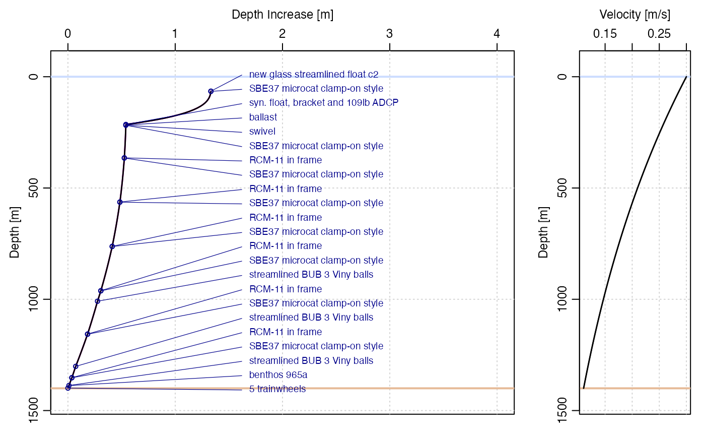
Figure 2. Simulation of knockdown with a depth-decaying current.
Knockdown-Speed Diagram
We may get an idea of the overall response of the mooring to water
velocity by running simulations with a range of velocities. Noting that
the top of the mooring, from the surface to 200m, is knocked over much
more than the rest, let’s focus on the depth of the second microcat from
the top, i.e. the one below the ADCP. Typing ms in a
console gives an overview, from which one may find the ADCP element
using
## [1] 23We may use this to construct a diagnostic curve giving an overview of the mooring knockdown, as follows. Note that the axis of the resultant plot is showing velocity at the depth of the ADCP.
par(mar = c(3, 3, 1, 1), mgp = c(2, 0.7, 0), mfrow = c(1, 1))
N <- 20
u0 <- seq(0, 0.3, length.out = N)
dz <- rep(NA, N)
U <- rep(NA, N)
for (i in seq_len(N)) {
    u <- function(depth) u0[i] * exp(-depth / 1400)
    k <- knockdown(ms, u)
    U[i] <- u(-k@elements[[iADCP]]@z)
    dz[i] <- k@elements[[iADCP]]@z - ms@elements[[iADCP]]@z
}
plot(U, dz, lwd = 2, type = "l", xlab = "Velocity [m/s]", ylab = "Knockdown [m]")
grid()
mtext(sprintf("Knockdown for ADCP nominally at %.0f m depth", -ms@elements[[iADCP]]@z))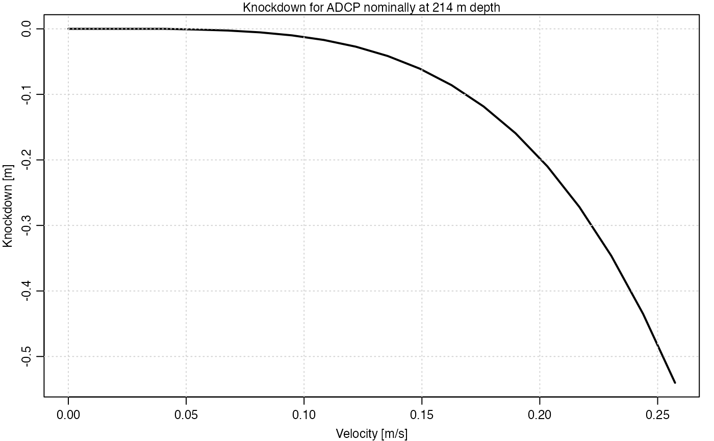
Figure 3. Speed-knockdown summary diagram
Examining Moorings
Overview
An overview of a mooring is provided by printing it, either with
print(m)or, in an interactive session, with
mNote that the results for ms will be similar, except
there will be many more elements (for the segmented chain and wire
components). If msk is examined in this way, the
and
values will be different.
Components
To learn more about, say, the top element, use
m@elements[[1]]## <mooring::floatS7>
## @ model : chr "new glass streamlined float c2"
## @ buoyancy : num 45.4
## @ height : num 0.87
## @ area : num 0.183
## @ CD : num 0.6
## @ source : chr "BIO"
## @ originalName: chr "NEW GLASS STREAMLINED FLOAT (C2)"
## @ x : num 0
## @ x0 : num 0
## @ z : num -63.6
## @ z0 : num -63.6
## @ phi : num 0
## @ tau : num 45.4
## @ group : num 0and, as shown previously, finer-grained access is achieved as, e.g.
m@elements[[1]]@buoyancy## [1] 45.41Exercise 1. Double the chain density, to see the effect on knock-down.
Exercise 2. Double the drag coefficient on the wire, to see how much this increases knockdown.
Answers to Exercises
1. Doubling chain density
A simple way to do this is to create m as before, but
then to use
m@elements[[2]]@buoyancy <- 2 * m@elements[[2]]@buoyancybefore using digitise(), knockdown() and
then plot.mooring(). Before doing that though, you should
ask yourself whether you expect to see a large effect.
2. Doubling wire drag
One way to do this is to replace the W definition
with
W <- function(length) {
    w0 <- wire("3/16in galvanized wire coated to 1/4in", length = 1)
    wire("draggy wire",
        buoyancy = w0@buoyancy,
        area = w0@area, CD = 2 * w0@CD, length = length
    )
}
and then create m, ms and msk
as before. The results are as follows. Note that an axis change is
required to capture the approximately-doubled knockdown. This
illustrates the importance of getting drag coefficient right, a matter
dealt with in detail by Hamilton (1989)
and Hamilton, Fowler, and Belliveau
(1997).
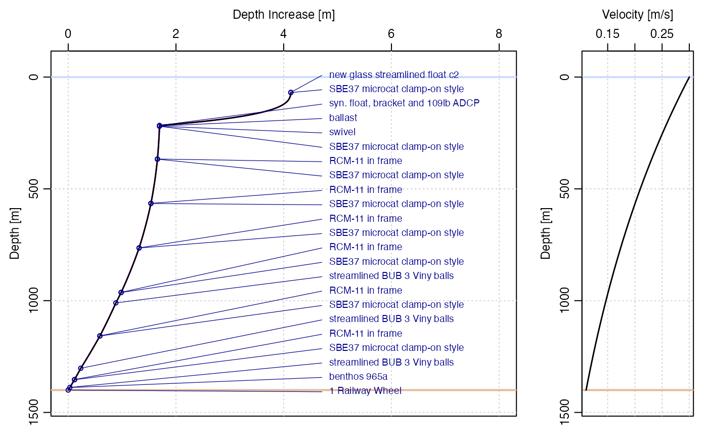
Figure 4. As Figure 2, but doubled wire drag. Note the doubled range of the ‘Depth Increase’ axis, to accomodate the approximately doubled knockdown.