Plot an echosounder Object

Plot echosounder data. Simple linear approximation is used when a newx value is specified with the which=2 method, but arguably a gridding method should be used, and this may be added in the future.

Usage

# S4 method for class 'echosounder'
plot(
  x,
  which = 1,
  beam = "a",
  newx,
  xlab,
  ylab,
  xlim,
  ylim,
  zlim,
  type = "l",
  col,
  lwd = 2,
  despike = FALSE,
  drawBottom,
  ignore = 5,
  drawTimeRange = FALSE,
  drawPalette = TRUE,
  radius,
  coastline,
  mgp = getOption("oceMgp"),
  mar = c(mgp[1], mgp[1] + 1.5, mgp[2] + 1/2, 1/2),
  atTop,
  labelsTop,
  tformat,
  debug = getOption("oceDebug"),
  ...
)

Arguments

x: an echosounder object.
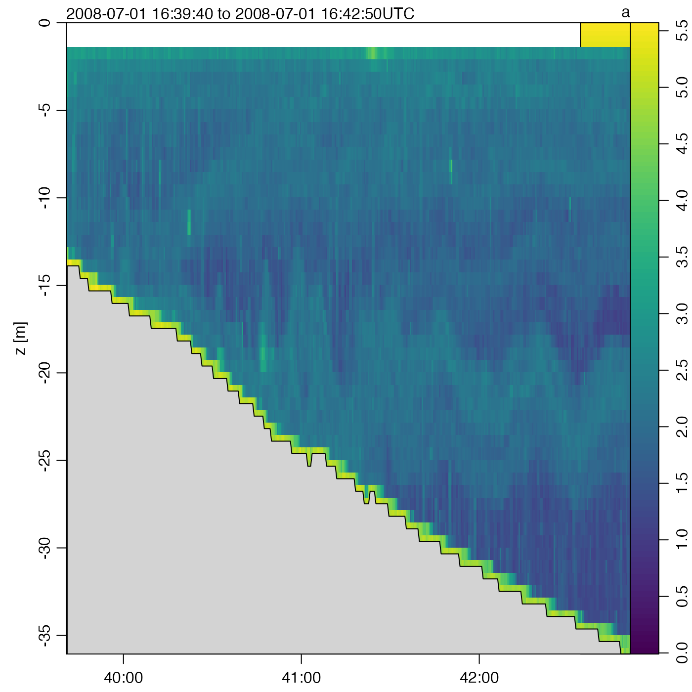
which: list of desired plot types: which=1 or which="zt image" gives a z-time image, which=2 or which="zx image" gives a z-distance image, and which=3 or which="map" gives a map showing the cruise track. In the image plots, the display is of log10() of amplitude, trimmed to zero for any amplitude values less than 1 (including missing values, which equal 0). Add 10 to the numeric codes to get the secondary data (non-existent for single-beam files,
beam: a more detailed specification of the data to be plotted. For single-beam data, this may only be "a". For dual-beam data, this may be "a" for the narrow-beam signal, or "b" for the wide-beam signal. For split-beam data, this may be "a" for amplitude, "b" for x-angle data, or "c" for y-angle data.
newx: optional vector of values to appear on the horizontal axis if which=1, instead of time. This must be of the same length as the time vector, because the image is remapped from time to newx using approx().
xlab, ylab: optional labels for the horizontal and vertical axes; if not provided, the labels depend on the value of which.
xlim: optional range for x axis.
ylim: optional range for y axis.
zlim: optional range for color scale.
type: type of graph, "l" for line, "p" for points, or "b" for both.
col: a function providing the color scale for image plots. This value is passed to imagep(), which draws the images. Since imagep() defaults col to oceColorsViridis(), that is effectively also the default for the present function. (Prior to 2023-03-18, the present function defaulted col to oceColorsJet().)
lwd: line width (ignored if type="p").
despike: remove vertical banding by using smooth() to smooth across image columns, row by row.
drawBottom: optional flag used for section images. If TRUE, then the bottom is inferred as a smoothed version of the ridge of highest image value, and data below that are grayed out after the image is drawn. If drawBottom is a color, then that color is used, instead of white. The bottom is detected with findBottom(), using the ignore value described next.
ignore: optional flag specifying the thickness in metres of a surface region to be ignored during the bottom-detection process. This is ignored unless drawBottom=TRUE.
drawTimeRange: if TRUE, the time range will be drawn at the top. Ignored except for which=2, i.e. distance-depth plots.
drawPalette: if TRUE, the palette will be drawn.
radius: radius to use for maps; ignored unless which=3 or which="map".
coastline: coastline to use for maps; ignored unless which=3 or which="map".
mgp: 3-element numerical vector to use for par("mgp"), and also for par("mar"), computed from this. The default is tighter than the R default, in order to use more space for the data and less for the axes.
mar: value to be used with par("mar").
atTop: optional vector of time values, for labels at the top of the plot produced with which=2. If labelsTop is provided, then it will hold the labels. If labelsTop is not provided, the labels will be constructed with the format() function, and these may be customized by supplying a format in the ... arguments.
labelsTop: optional vector of character strings to be plotted above the atTop times. Ignored unless atTop was provided.
tformat: optional argument passed to imagep(), for plot types that call that function. (See strptime() for the format used.)
debug: set to an integer exceeding zero, to get debugging information during processing.
...: optional arguments passed to plotting functions. For example, for maps, it is possible to specify the radius of the view in kilometres, with radius.

Value

A list is silently returned, containing xat and yat, values that can be used by oce.grid() to add a grid to the plot.

Author

Dan Kelley, with extensive help from Clark Richards

Examples

library(oce)
data(echosounder)
plot(echosounder, drawBottom = TRUE)

Usage

Arguments

Value

See also

Author

Examples