Oce Variant of contour — oce.contour • oce

This provides something analogous to contour(), but with the ability to flip x and y. Setting revy=TRUE can be helpful if the y data represent pressure or depth below the surface.

Usage

oce.contour(
  x,
  y,
  z,
  revx = FALSE,
  revy = FALSE,
  add = FALSE,
  tformat,
  drawTimeRange = getOption("oceDrawTimeRange"),
  debug = getOption("oceDebug"),
  ...
)

Arguments

x: values for x grid.
y: values for y grid.
z: matrix for values to be contoured. The first dimension of z must equal the number of items in x, etc.
revx: set to TRUE to reverse the order in which the labels on the x axis are drawn
revy: set to TRUE to reverse the order in which the labels on the y axis are drawn
add: logical value indicating whether the contours should be added to a pre-existing plot.
tformat: time format; if not supplied, a reasonable choice will be made by oce.axis.POSIXct(), which draws time axes.
drawTimeRange: logical, only used if the x axis is a time. If TRUE, then an indication of the time range of the data (not the axis) is indicated at the top-left margin of the graph. This is useful because the labels on time axes only indicate hours if the range is less than a day, etc.
debug: a flag that turns on debugging; set to 1 to information about the processing.
...: optional arguments passed to plotting functions.

Author

Dan Kelley

Examples

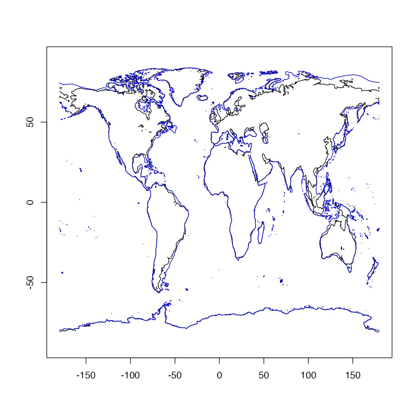
library(oce)
data(topoWorld)
# coastline now, and in last glacial maximum
lon <- topoWorld[["longitude"]]
lat <- topoWorld[["latitude"]]
z <- topoWorld[["z"]]
oce.contour(lon, lat, z, levels = 0, drawlabels = FALSE)
oce.contour(lon, lat, z, levels = -130, drawlabels = FALSE, col = "blue", add = TRUE)