Make a Digital Filter

The filter is suitable for use by filter(), convolve() or (for the asKernal=TRUE case) with kernapply(). Note that convolve() should be faster than filter(), but it cannot be used if the time series has missing values. For the Blackman-Harris filter, the half-power frequency is at 1/m cycles per time unit, as shown in the “Examples” section. When using filter() or kernapply() with these filters, use circular=TRUE.

makeFilter(
  type = c("blackman-harris", "rectangular", "hamming", "hann"),
  m,
  asKernel = TRUE
)

Arguments

type

a string indicating the type of filter to use. (See Harris (1978) for a comparison of these and similar filters.)

• "blackman-harris" yields a modified raised-cosine filter designated as "4-Term (-92 dB) Blackman-Harris" by Harris (1978; coefficients given in the table on page 65). This is also called "minimum 4-sample Blackman Harris" by that author, in his Table 1, which lists figures of merit as follows: highest side lobe level -92dB; side lobe fall off -6 db/octave; coherent gain 0.36; equivalent noise bandwidth 2.00 bins; 3.0-dB bandwidth 1.90 bins; scallop loss 0.83 dB; worst case process loss 3.85 dB; 6.0-db bandwidth 2.72 bins; overlap correlation 46 percent for 75\ for 50\ a spectral peak, so that a value of 2 indicates a cutoff frequency of 1/m, where m is as given below.

• "rectangular" for a flat filter. (This is just for convenience. Note that kernel("daniell",....) gives the same result, in kernel form.) "hamming" for a Hamming filter (a raised-cosine that does not taper to zero at the ends)

• "hann" (a raised cosine that tapers to zero at the ends).

m

length of filter. This should be an odd number, for any non-rectangular filter.

asKernel

boolean, set to TRUE to get a smoothing kernel for the return value.

Value

If asKernel is FALSE, this returns a list of filter coefficients, symmetric about the midpoint and summing to 1. These may be used with filter(), which should be provided with argument circular=TRUE to avoid phase offsets. If asKernel is TRUE, the return value is a smoothing kernel, which can be applied to a timeseries with kernapply(), whose bandwidth can be determined with bandwidth.kernel(), and which has both print and plot methods.

Sample of Usage

# need signal package for this example
r <- rnorm(2048)
rh <- stats::filter(r, H)
rh <- rh[is.finite(rh)] # kludge to remove NA at start/end
sR <- spectrum(r, plot=FALSE, spans=c(11, 5, 3))
sRH <- spectrum(rh, plot=FALSE, spans=c(11, 5, 3))
par(mfrow=c(2, 1), mar=c(3, 3, 1, 1), mgp=c(2, 0.7, 0))
plot(sR$freq, sRH$spec/sR$spec, xlab="Frequency", ylab="Power Transfer",
     type="l", lwd=5, col="gray")
theory <- freqz(H, n=seq(0,pi,length.out=100))
# Note we must square the modulus for the power spectrum
lines(theory$f/pi/2, Mod(theory$h)^2, lwd=1, col="red")
grid()
legend("topright", col=c("gray", "red"), lwd=c(5, 1), cex=2/3,
       legend=c("Practical", "Theory"), bg="white")
plot(log10(sR$freq), log10(sRH$spec/sR$spec),
     xlab="log10 Frequency", ylab="log10 Power Transfer",
     type="l", lwd=5, col="gray")
theory <- freqz(H, n=seq(0,pi,length.out=100))
# Note we must square the modulus for the power spectrum
lines(log10(theory$f/pi/2), log10(Mod(theory$h)^2), lwd=1, col="red")
grid()
legend("topright", col=c("gray", "red"), lwd=c(5, 1), cex=2/3,
       legend=c("Practical", "Theory"), bg="white")

References

F. J. Harris, 1978. On the use of windows for harmonic analysis with the discrete Fourier Transform. Proceedings of the IEEE, 66(1), 51-83 (http://web.mit.edu/xiphmont/Public/windows.pdf.)

Author

Dan Kelley

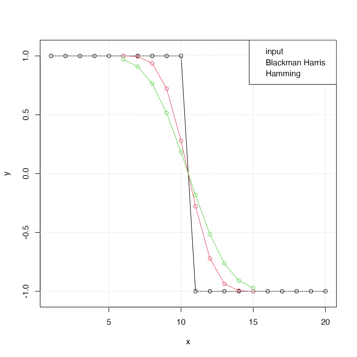
Examples

library(oce)

# 1. Demonstrate step-function response
y <- c(rep(1, 10), rep(-1, 10))
x <- seq_along(y)
plot(x, y, type = "o", ylim = c(-1.05, 1.05))
BH <- makeFilter("blackman-harris", 11, asKernel = FALSE)
H <- makeFilter("hamming", 11, asKernel = FALSE)
yBH <- stats::filter(y, BH)
points(x, yBH, col = 2, type = "o")
yH <- stats::filter(y, H)
points(yH, col = 3, type = "o")
legend("topright",
    col = 1:3, cex = 2 / 3, pch = 1,
    legend = c("input", "Blackman Harris", "Hamming")
)


# 2. Show theoretical and practical filter gain, where
#    the latter is based on random white noise, and
#    includes a particular value for the spans
#    argument of spectrum(), etc.