Welch Periodogram — pwelch • oce

Compute periodogram using the Welch (1967) method. This function is somewhat analogous to the Matlab function of the same name, but it is not intended as a drop-in replacement. Please see the ‘Arguments’ and ‘Details’ to learn about the complex interactions of the controlling parameters.

Usage

pwelch(
  x,
  window,
  noverlap,
  nfft,
  fs,
  spec,
  demean = FALSE,
  detrend = TRUE,
  plot = TRUE,
  debug = getOption("oceDebug"),
  ...
)

Arguments

x: a vector or timeseries to be analyzed. If x is a timeseries, then it there is no need to fs, and doing so will result in an error if it does not match the value inferred from x.
window: optional value that can have several meanings. CASE 1: If window is a single integer, then that is taken as the number of fragments into which x is subdivided. In this case, a Hamming window, of length length(x)/window, is constructed using makeFilter() with its normalize and asKernel arguments both set to FALSE. This filter is then multiplied elementwise with the x values in the subdivision. CASE 2: if window is a numeric vector of length exceeding 1, then the values are taken to be a filter to be applied to the subset of x, and thus the length of window and the value of nfft must be equal, if both are supplied.
noverlap: number of points to overlap between the subdivisions of x. If this is not provided, a value equal to half the subset length will be used.
nfft: length of the FFT, i.e. length of the desired subsets of x. This argument works together with the window argument; see the documentation on the latter to learn more.
fs: numeric value indicating the sampling frequency for x. If x is already a time-series object, then fs must match its frequency, or an error is reported.
spec: optional function to be used, in conjunction with nfft, to control the computation of the spectra in the subdivided time-series. The purpose is to allow fine-grained control of the processing, mainly for use by experts. If provided, spec must accept a time-series as its first argument, along with optional other arguments that are passed through as the ... argument. The return value from spec must be a list or data frame containing the spectrum in an element named spec and the frequency in an element named freq. Note that an error will be reported if window is provided in addition to spec and nfft. This is because pwelch() automatically constructs a (Hamming) window and multiplies it into each subset of x. Also, note that the values of demean and detrend are ignored if spec is provided; it's up to the user to decide on these things and to handle them within spec().
demean, detrend: logical values that can control the spectrum calculation, but only if spec is not provided. These are passed to spectrum() and thence to spec.pgram(); see the help pages for the latter for an explanation.
plot: logical, set to TRUE to plot the spectrum.
debug: a flag that turns on debugging. Set to 1 to get a moderate amount of debugging information, or to 2 to get more.
...: optional extra arguments to be passed to spectrum(), or to spec, if the latter is given.

Value

pwelch returns a list mimicking the return value from spectrum(), containing frequency freq, spectral power spec, degrees of freedom df, bandwidth bandwidth, etc.

Details

The gist of the pwelch() behaviour is not too difficult to explain: x is broken up into subdivisions, spectral analysis is done on each, and the results are averaged to get a return value.

However, things get complicated in practice. This is because there are several interlocking parameters that control both the subdivision stage and the spectral stage. The goal is to at least roughly mimic the Matlab function, so the parameter names and how they are interpreted are dictated to some extent by how things work in the Matlab code.

The parameters window, noverlap and nfft control the subdivision behaviour. The parameters fs, spec, demean and detrend control the spectral-analysis behaviour. Users who find the documentation on these things to be confusing may want to examine the code to see what is actually being done. If they see problems, they are asked to post issues on the oce github website.

Bugs

Both bandwidth and degrees of freedom are just copied from the values for one of the chunk spectra, and are thus incorrect. That means the cross indicated on the graph is also incorrect.

Historical notes

2021-06-26: Until this date, pwelch() passed the subsampled timeseries portions through detrend() before applying the window. This practice was dropped because it could lead to over-estimates of low frequency energy (as noticed by Holger Foysi of the University of Siegen), perhaps because detrend() considers only endpoints and therefore can yield inaccurate trend estimates. In a related change, demean and detrend were added as formal arguments, to avoid users having to trace the documentation for spectrum() and then spec.pgram(), to learn how to remove means and trends from data. For more control, the spec argument was added to let users sidestep spectrum() entirely, by providing their own spectral computation functions.
2025-07-04: until this date, there was an error in supplying nfft together with spec (it is issue 2299 on the github website). This issued an error message that resulted from the fact that it was not permitted to supply window in that case. To address the problem, whilst retaining the requirement that window not be supplied, pwelch() was changed so that it constructs a window automatically. (In the future, pwelch() may be modified to accept window=FALSE, in which case no windowing will be done here, leaving it up to the user to decide whether to do windowing in the user-supplied spec() function.)

References

Welch, P. D., 1967. The Use of Fast Fourier Transform for the Estimation of Power Spectra: A Method Based on Time Averaging Over Short, Modified Periodograms. IEEE Transactions on Audio Electroacoustics, AU-15, 70–73.

Author

Dan Kelley and Clark Richards

Examples

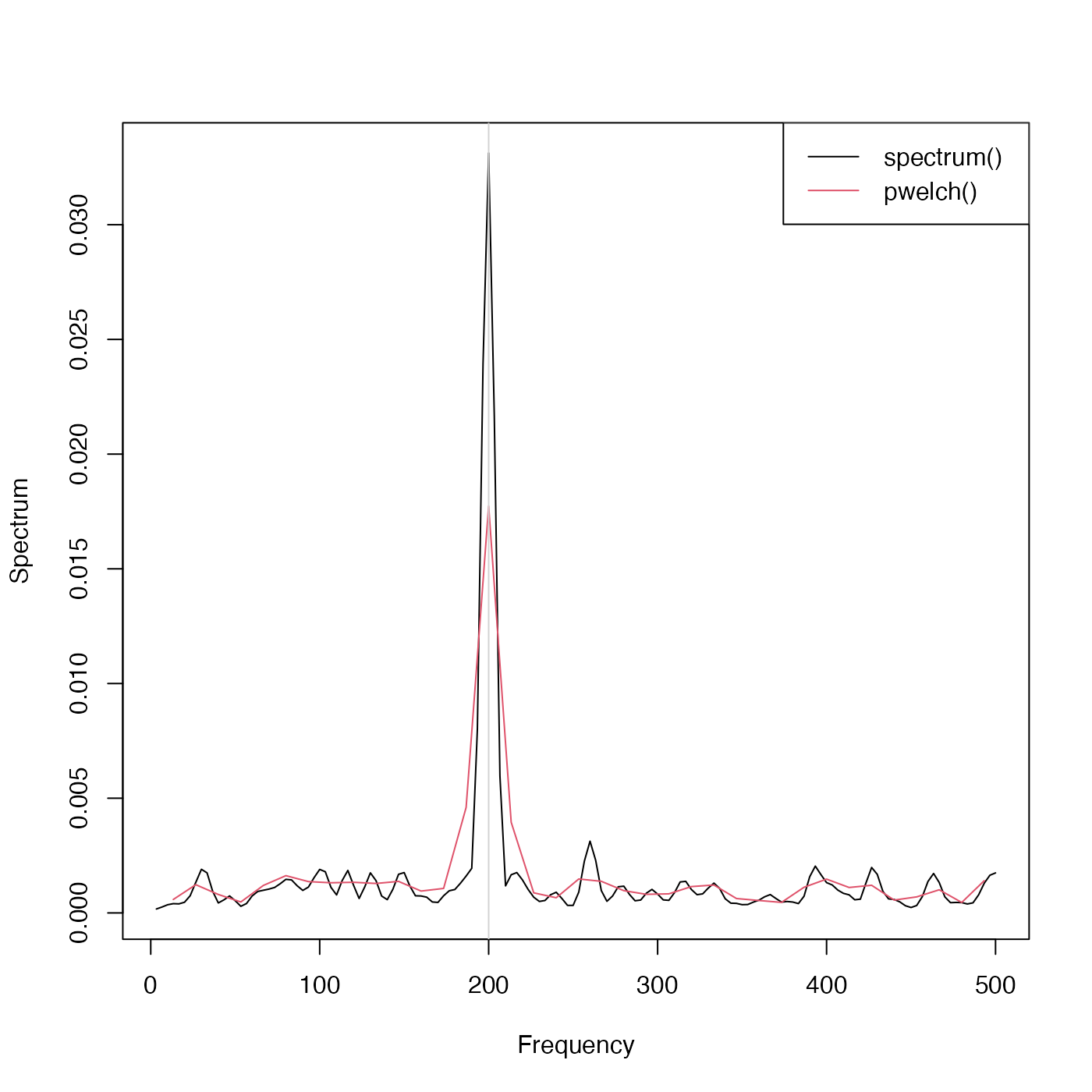
library(oce)
Fs <- 1000
t <- seq(0, 0.296, 1 / Fs)
x <- cos(2 * pi * t * 200) + rnorm(n = length(t))
X <- ts(x, frequency = Fs)
s <- spectrum(X, spans = c(3, 2), log = "no", plot = FALSE)
plot(s$freq, s$spec, type = "l", xlab = "Frequency", ylab = "Spectrum")
w <- pwelch(X, plot = FALSE)
lines(w$freq, w$spec, col = 2)
abline(v = 200, col = "lightgray")
legend("topright", bg = "white", lwd = 1, col = 1:2, legend = c("spectrum()", "pwelch()"))