Earth Magnetic Declination, Inclination, and Intensity

Implements the 12th and 13th generations of the International Geomagnetic Reference Field (IGRF), based on a reworked version of a Fortran program downloaded from a NOAA website (see “References”).

magneticField(longitude, latitude, time, version = 13)

Arguments

longitude: longitude in degrees east (negative for degrees west), as a number, a vector, or a matrix.
latitude: latitude in degrees north, as a number, vector, or matrix. The shape (length or dimensions) must conform to the dimensions of longitude.
time: The time at which the field is desired. This may be a single value or a vector or matrix that is structured to match longitude and latitude. The value may a decimal year, a POSIXt time, or a Date time.
version: an integer that must be either 12 or 13, to specify the version number of the formulae. Note that 13 became the default on 2020 March 3, so to old code will need to specify version=12 to work as it did before that date.

Value

A list containing declination, inclination, and intensity.

Details

The code (subroutines igrf12syn and igrf13syn) seem to have been written by Susan Macmillan of the British Geological Survey. Comments in the source code igrf13syn (the current default used here) indicate that its coefficients were agreed to in December 2019 by the IAGA Working Group V-MOD. Other comments in that code suggest that the proposed application time interval is from years 1900 to 2025, inclusive, but that only dates from 1945 to 2015 are to be considered definitive.

Historical Notes

For about a decade, magneticField used the version 12 formulae provided by IAGA, but the code was updated on March 3, 2020, to version 13. Example 3 shows that the differences in declination are typically under 2 degrees (with 95 percent of the data lying between -1.7 and 0.7 degrees).

References

The underlying Fortran code for version 12 is from igrf12.f, downloaded the NOAA website (https://www.ngdc.noaa.gov/IAGA/vmod/igrf.html) on June 7,
That for version 13 is igrf13.f, downloaded from the NOAA website (https://www.ngdc.noaa.gov/IAGA/vmod/igrf.html on March 3, 2020.
Witze, Alexandra. “Earth's Magnetic Field Is Acting up and Geologists Don't Know Why.” Nature 565 (January 9, 2019): 143. doi:10.1038/d41586-019-00007-1
Alken, P., E. Thébault, C. D. Beggan, H. Amit, J. Aubert, J. Baerenzung, T. N. Bondar, et al. "International Geomagnetic Reference Field: The Thirteenth Generation." Earth, Planets and Space 73, no. 1 (December 2021): 49. doi:10.1186/s40623-020-01288-x .

Author

Dan Kelley wrote the R code and a fortran wrapper to the igrf12.f subroutine, which was written by Susan Macmillan of the British Geological Survey and distributed ``without limitation'' (email from SM to DK dated June 5, 2015). This version was updated subsequent to that date; see “Historical Notes”.

Examples

library(oce)
# 1. Today's value at Halifax NS
magneticField(-(63 + 36 / 60), 44 + 39 / 60, Sys.Date())
#> $declination
#> [1] -16.39477
#> 
#> $inclination
#> [1] 66.45537
#> 
#> $intensity
#> [1] 51234.46
#> 

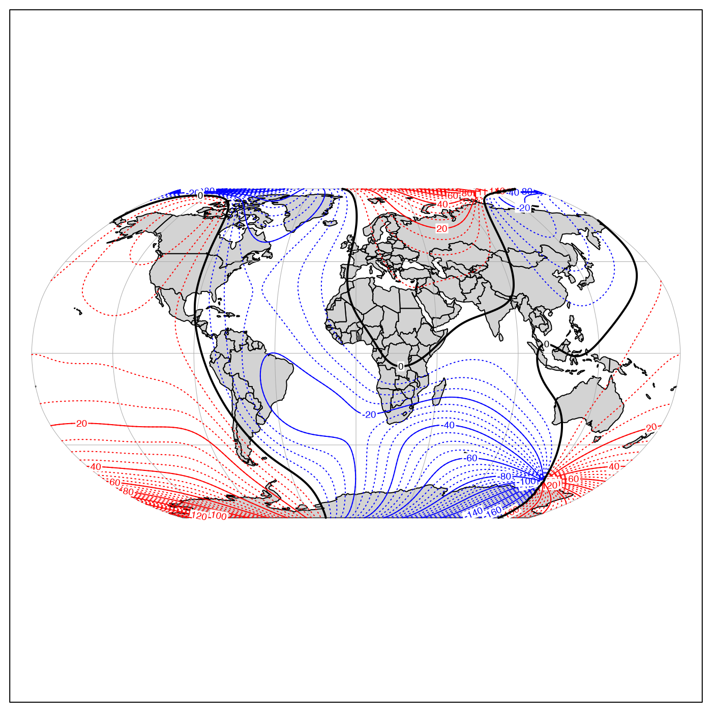
# 2. World map of declination in year 2000.
# \donttest{
data(coastlineWorld)
par(mar = rep(0.5, 4)) # no axes on whole-world projection
mapPlot(coastlineWorld, projection = "+proj=robin", col = "lightgray")
# Construct matrix holding declination
lon <- seq(-180, 180)
lat <- seq(-90, 90)
dec2000 <- function(lon, lat) {
    magneticField(lon, lat, 2000)$declination
}
dec <- outer(lon, lat, dec2000) # hint: outer() is very handy!
# Contour, unlabelled for small increments, labeled for
# larger increments.
mapContour(lon, lat, dec,
    col = "blue", levels = seq(-180, -5, 5),
    lty = 3, drawlabels = FALSE
)
mapContour(lon, lat, dec, col = "blue", levels = seq(-180, -20, 20))
mapContour(lon, lat, dec,
    col = "red", levels = seq(5, 180, 5),
    lty = 3, drawlabels = FALSE
)
mapContour(lon, lat, dec, col = "red", levels = seq(20, 180, 20))
mapContour(lon, lat, dec, levels = 180, col = "black", lwd = 2, drawlabels = FALSE)
mapContour(lon, lat, dec, levels = 0, col = "black", lwd = 2)

# }

# 3. Declination differences between versions 12 and 13
# \donttest{
lon <- seq(-180, 180)
lat <- seq(-90, 90)
decDiff <- function(lon, lat) {
    old <- magneticField(lon, lat, 2020, version = 13)$declination
    new <- magneticField(lon, lat, 2020, version = 12)$declination
    new - old
}
decDiff <- outer(lon, lat, decDiff)
decDiff <- ifelse(decDiff > 180, decDiff - 360, decDiff)
# Overall (mean) shift -0.1deg
t.test(decDiff)
#> 
#> 	One Sample t-test
#> 
#> data:  decDiff
#> t = -21.794, df = 65340, p-value < 2.2e-16
#> alternative hypothesis: true mean is not equal to 0
#> 95 percent confidence interval:
#>  -0.10399320 -0.08683188
#> sample estimates:
#>   mean of x 
#> -0.09541254 
#> 
# View histogram, narrowed to small differences
par(mar = c(3.5, 3.5, 2, 2), mgp = c(2, 0.7, 0))
hist(decDiff,
    breaks = seq(-180, 180, 0.05), xlim = c(-2, 2),
    xlab = "Declination difference [deg] from version=12 to version=13",
    main = "Predictions for year 2020"
)

print(quantile(decDiff, c(0.025, 0.975)))
#>       2.5%      97.5% 
#> -1.6695352  0.7159345 
# Note that the large differences are at high latitudes
imagep(lon, lat, decDiff, zlim = c(-1, 1) * max(abs(decDiff)))
lines(coastlineWorld[["longitude"]], coastlineWorld[["latitude"]])

# }