In the interior of the matrix, centred second-order differences are used to infer the components of the grad. Along the edges, first-order differences are used.
Value
A list containing \(|\nabla h|\) as g,
\(\partial h/\partial x\) as gx,
and \(\partial h/\partial y\) as gy,
each of which is a matrix of the same dimension as h.
See also
Other things relating to vector calculus:
curl()
Examples
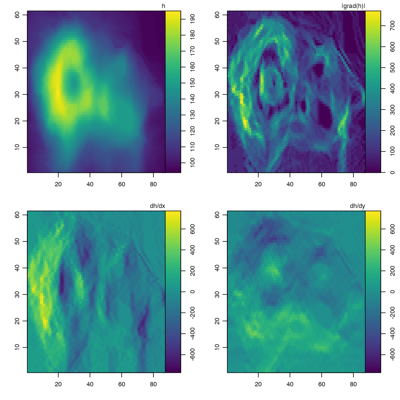
# 1. Built-in volcano dataset
g <- grad(volcano)
par(mfrow = c(2, 2), mar = c(3, 3, 1, 1), mgp = c(2, 0.7, 0))
imagep(volcano, zlab = "h")
imagep(g$g, zlab = "|grad(h)|")
zlim <- c(-1, 1) * max(g$g)
imagep(g$gx, zlab = "dh/dx", zlim = zlim)
imagep(g$gy, zlab = "dh/dy", zlim = zlim)


# 2. Geostrophic flow around an eddy
library(oce)
dx <- 5e3
dy <- 10e3
x <- seq(-200e3, 200e3, dx)
y <- seq(-200e3, 200e3, dy)
R <- 100e3
h <- outer(x, y, function(x, y) 500 * exp(-(x^2 + y^2) / R^2))
grad <- grad(h, x, y)
par(mfrow = c(2, 2), mar = c(3, 3, 1, 1), mgp = c(2, 0.7, 0))
contour(x, y, h, asp = 1, main = expression(h))
f <- 1e-4
gprime <- 9.8 * 1 / 1024
u <- -(gprime / f) * grad$gy
v <- (gprime / f) * grad$gx
contour(x, y, u, asp = 1, main = expression(u))
contour(x, y, v, asp = 1, main = expression(v))
contour(x, y, sqrt(u^2 + v^2), asp = 1, main = expression(speed))
