Curl of 2D Vector Field

Calculate the z component of the curl of an x-y vector field.

curl(u, v, x, y, geographical = FALSE, method = 1)

Arguments

u: matrix containing the 'x' component of a vector field
v: matrix containing the 'y' component of a vector field
x: the x values for the matrices, a vector of length equal to the number of rows in u and v.
y: the y values for the matrices, a vector of length equal to the number of cols in u and v.
geographical: logical value indicating whether x and y are longitude and latitude, in which case spherical trigonometry is used.
method: A number indicating the method to be used to calculate the first-difference approximations to the derivatives. See “Details”.

Value

A list containing vectors x and y, along with matrix curl. See “Details” for the lengths and dimensions, for various values of method.

Details

The computed component of the curl is defined by \(\partial \)\( v/\partial x - \partial u/\partial y\) and the estimate is made using first-difference approximations to the derivatives. Two methods are provided, selected by the value of method.

For method=1, a centred-difference, 5-point stencil is used in the interior of the domain. For example, \(\partial v/\partial x\) is given by the ratio of \(v_{i+1,j}-v_{i-1,j}\) to the x extent of the grid cell at index \(j\). (The cell extents depend on the value of geographical.) Then, the edges are filled in with nearest-neighbour values. Finally, the corners are filled in with the adjacent value along a diagonal. If geographical=TRUE, then x and y are taken to be longitude and latitude in degrees, and the earth shape is approximated as a sphere with radius 6371km. The resultant x and y are identical to the provided values, and the resultant curl is a matrix with dimension identical to that of u.
For method=2, each interior cell in the grid is considered individually, with derivatives calculated at the cell center. For example, \(\partial v/\partial x\) is given by the ratio of \(0.5*(v_{i+1,j}+v_{i+1,j+1}) - 0.5*(v_{i,j}+v_{i,j+1})\) to the average of the x extent of the grid cell at indices \(j\) and \(j+1\). (The cell extents depend on the value of geographical.) The returned x and y values are the mid-points of the supplied values. Thus, the returned x and y are shorter than the supplied values by 1 item, and the returned curl matrix dimensions are similarly reduced compared with the dimensions of u and v.

Author

Dan Kelley and Chantelle Layton

Examples

library(oce)
# 1. Shear flow with uniform curl.
x <- 1:4
y <- 1:10
u <- outer(x, y, function(x, y) y / 2)
v <- outer(x, y, function(x, y) -x / 2)
C <- curl(u, v, x, y, FALSE)

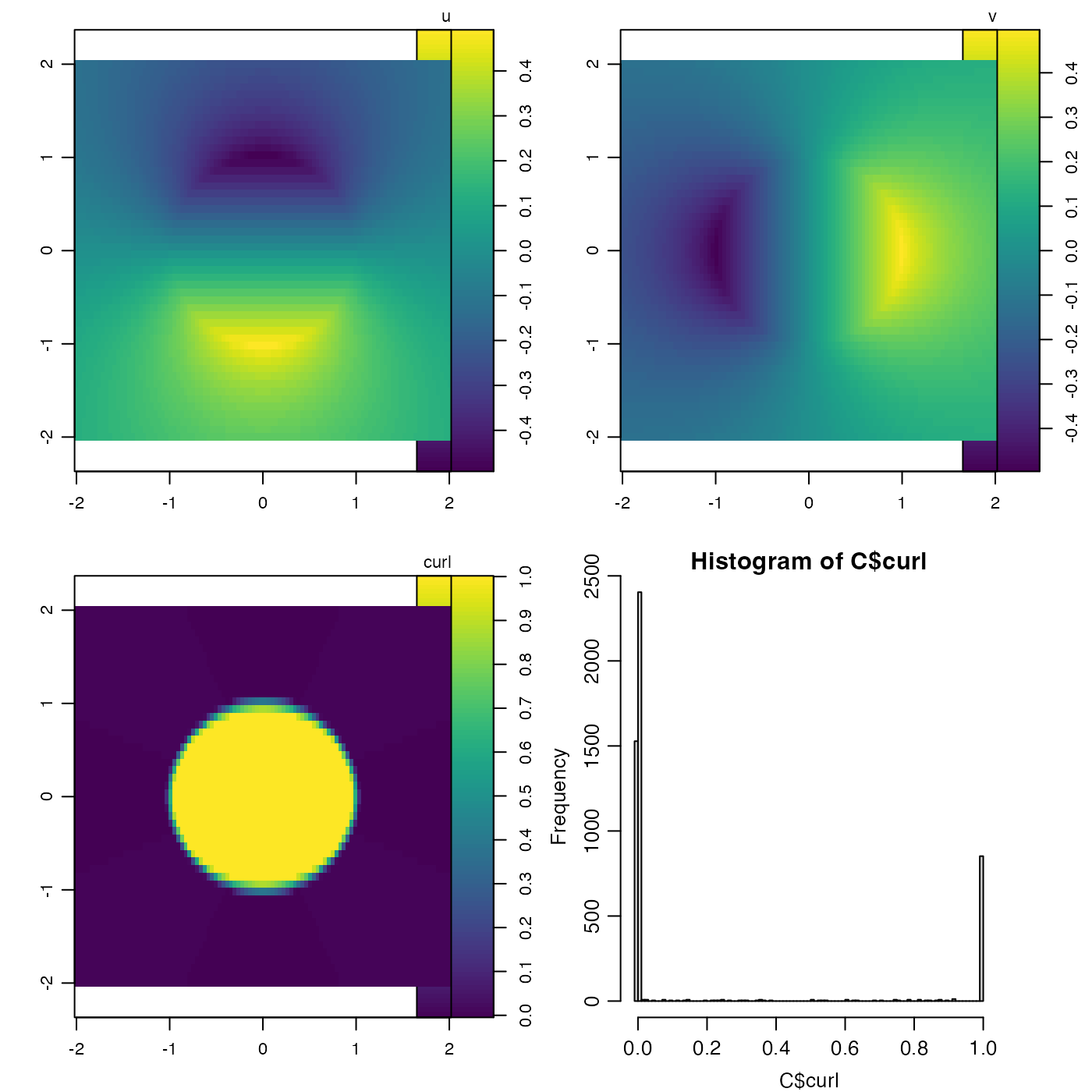
# 2. Rankine vortex: constant curl inside circle, zero outside
rankine <- function(x, y) {
    r <- sqrt(x^2 + y^2)
    theta <- atan2(y, x)
    speed <- ifelse(r < 1, 0.5 * r, 0.5 / r)
    list(u = -speed * sin(theta), v = speed * cos(theta))
}
x <- seq(-2, 2, length.out = 100)
y <- seq(-2, 2, length.out = 50)
u <- outer(x, y, function(x, y) rankine(x, y)$u)
v <- outer(x, y, function(x, y) rankine(x, y)$v)
C <- curl(u, v, x, y, FALSE)
# plot results
par(mfrow = c(2, 2))
imagep(x, y, u, zlab = "u", asp = 1)
imagep(x, y, v, zlab = "v", asp = 1)
imagep(x, y, C$curl, zlab = "curl", asp = 1)
hist(C$curl, breaks = 100)