The linear model is calculated from the slope of a localized least-squares
regression model y=y(x). The localization is defined by the x difference
from the point in question, with data at distance exceeding L/2 being
ignored. With a boxcar window, all data within the local domain are
treated equally, while with a hanning window, a raised-cosine
weighting function is used; the latter produces smoother derivatives, which
can be useful for noisy data. The function is based on internal
calculation, not on lm().
Usage
runlm(x, y, xout, window = c("hanning", "boxcar"), L, deriv)Arguments
- x
a vector holding x values.
- y
a vector holding y values.
- xout
optional vector of x values at which the derivative is to be found. If not provided,
xis used.- window
type of weighting function used to weight data within the window; see “Details”.
- L
width of running window, in x units. If not provided, a reasonable default will be used.
- deriv
an optional indicator of the desired return value; see “Examples”.
Value
If deriv is not specified, a list containing vectors of
output values y and y, derivative (dydx), along with
the scalar length scale L. If deriv=0, a vector of values is
returned, and if deriv=1, a vector of derivatives is returned.
Examples
library(oce)
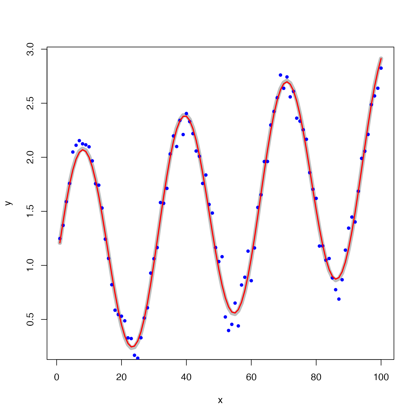
# Case 1: smooth a noisy signal
x <- 1:100
y <- 1 + x / 100 + sin(x / 5)
yn <- y + rnorm(100, sd = 0.1)
L <- 4
calc <- runlm(x, y, L = L)
plot(x, y, type = "l", lwd = 7, col = "gray")
points(x, yn, pch = 20, col = "blue")
lines(x, calc$y, lwd = 2, col = "red")
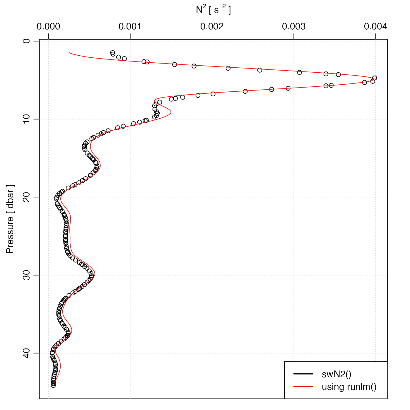
 # Case 2: square of buoyancy frequency
data(ctd)
par(mfrow = c(1, 1))
plot(ctd, which = "N2")
rho <- swRho(ctd)
z <- swZ(ctd)
zz <- seq(min(z), max(z), 0.1)
N2 <- -9.8 / mean(rho) * runlm(z, rho, zz, deriv = 1)
lines(N2, -zz, col = "red")
legend("bottomright",
lwd = 2, bg = "white",
col = c("black", "red"),
legend = c("swN2()", "using runlm()")
)
# Case 2: square of buoyancy frequency
data(ctd)
par(mfrow = c(1, 1))
plot(ctd, which = "N2")
rho <- swRho(ctd)
z <- swZ(ctd)
zz <- seq(min(z), max(z), 0.1)
N2 <- -9.8 / mean(rho) * runlm(z, rho, zz, deriv = 1)
lines(N2, -zz, col = "red")
legend("bottomright",
lwd = 2, bg = "white",
col = c("black", "red"),
legend = c("swN2()", "using runlm()")
)