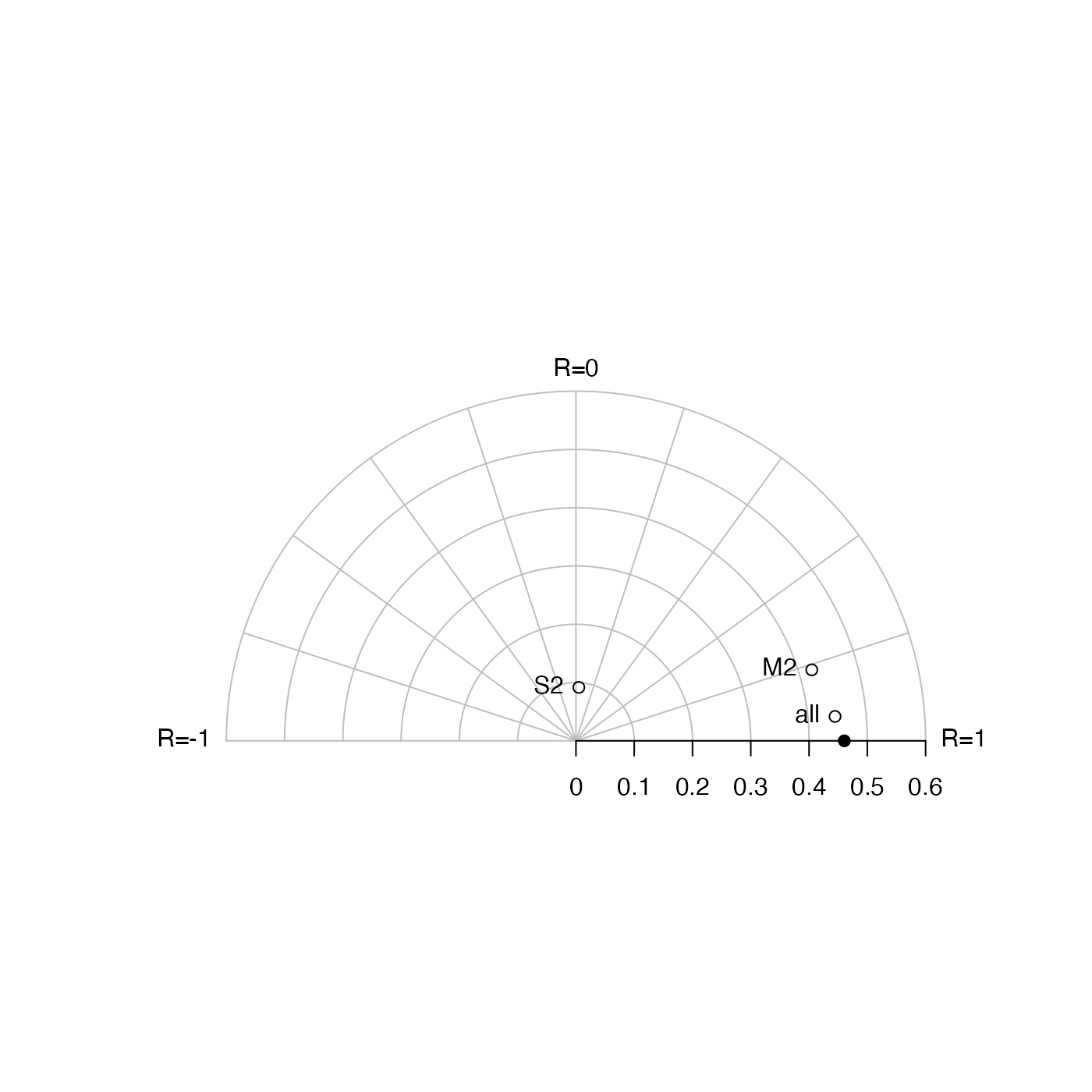
Creates a diagram as described by Taylor (2001). The graph is in the form of a semicircle, with radial lines and spokes connecting at a focus point on the flat (lower) edge. The radius of a point on the graph indicates the standard deviation of the corresponding quantity, i.e. x and the columns in y. The angle connecting a point on the graph to the focus provides an indication of correlation coefficient with respect to x.
Arguments
- x
a vector of reference values of some quantity, e.g. measured over time or space.
- y
a matrix whose columns hold values of values to be compared with those in x. (If
yis a vector, it is converted first to a one-column matrix).- scale
optional scale, interpreted as the maximum value of the standard deviation.
- pch
vector of plot symbols, used for points on the plot. If this is of length less than the number of columns in
y, then it it is repeated as needed to match those columns.- col
vector of colors for points on the plot, repeated as necessary (see
pch).- labels
optional vector of strings to use for labelling the points.
- pos
optional vector of positions for labelling strings, repeated as necessary (see
pch).- cex
character expansion factor, repeated if necessary (see
pch).
Details
The “east” side of the graph indicates \(R=1\), while
\(R=0\) is at the "north" edge and \(R=-1\) is at
the "west" side. The x data are indicated with a bullet on the
graph, appearing on the lower edge to the right of the focus at a
distance indicating the standard deviation of `x`. The other
points on the graph represent the columns of `y`, coded
automatically or with the supplied values of `pch` and `col`. The
example shows three tidal models of the Halifax sealevel data,
computed with tidem() with only the M2 component, only the S2
component, or all (auto-selected) components.
References
Taylor, Karl E. "Summarizing Multiple Aspects of Model Performance in a Single Diagram." Journal of Geophysical Research: Atmospheres 106, no. D7 (April 16, 2001): 7183–92. https://doi.org/10.1029/2000JD900719.
Examples
library(oce)
data(sealevel)
x <- sealevel[["elevation"]]
M2 <- predict(tidem(sealevel, constituents = "M2"))
S2 <- predict(tidem(sealevel, constituents = "S2"))
all <- predict(tidem(sealevel))
#> Warning: tidal record too short to fit constituents: SA, PI1, S1, PSI1, GAM2, H1, H2, T2, R2
plotTaylor(x, cbind(M2, S2, all), labels = c("M2", "S2", "all"))