Filter a Time Series

Filter a time-series, possibly recursively

oceFilter(x, a = 1, b, zero.phase = FALSE)

Arguments

x

a vector of numeric values, to be filtered as a time series.

a

a vector of numeric values, giving the \(a\) coefficients (see “Details”).

b

a vector of numeric values, giving the \(b\) coefficients (see “Details”).

zero.phase

boolean, set to TRUE to run the filter forwards, and then backwards, thus removing any phase shifts associated with the filter.

Value

A numeric vector of the filtered results, \(y\), as denoted in “Details”.

Details

The filter is defined as e.g. \(y[i]=b[1]*x[i] + \)\( b[2]*x[i-1] + b[3]*x[i-2] + ... - a[2]*y[i-1] - a[3]*y[i-2] - \)\( a[4]*y[i-3] - ...\), where some of the illustrated terms will be omitted if the lengths of a and b are too small, and terms are dropped at the start of the time series where the index on x would be less than 1.

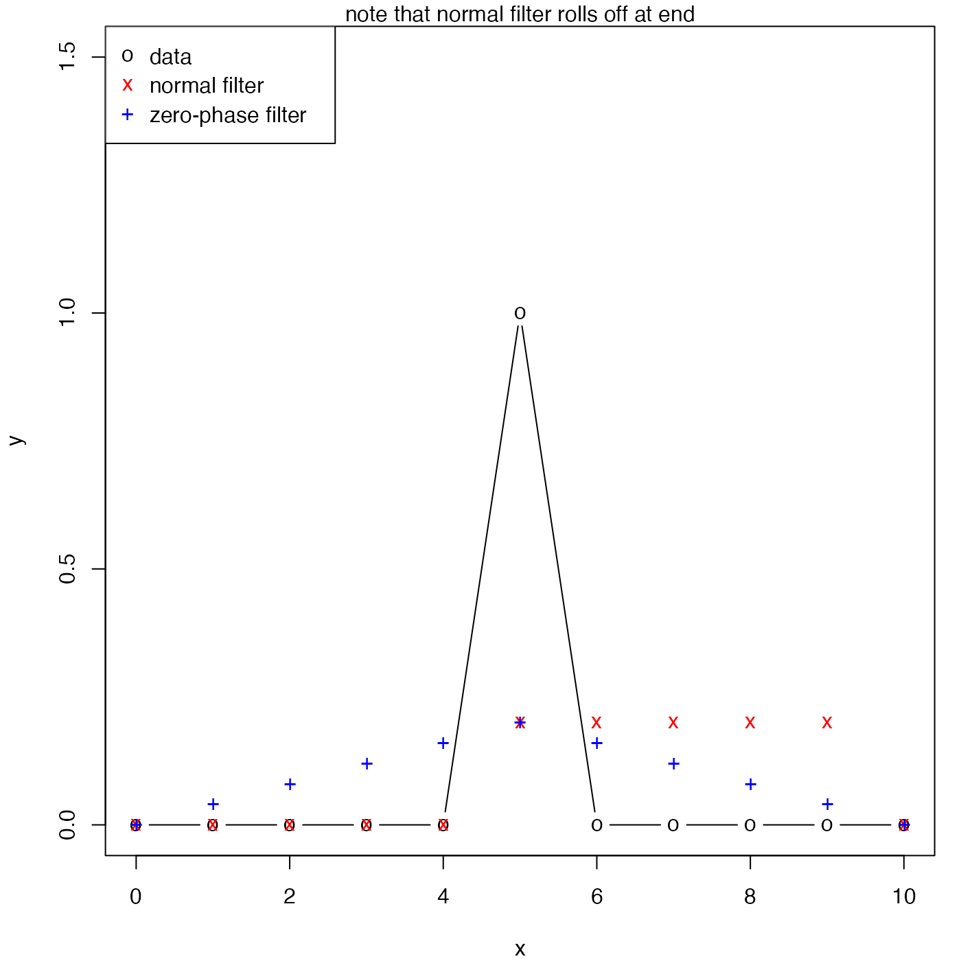
By contrast with the filter() function of R, oce.filter lacks the option to do a circular filter. As a consequence, oceFilter introduces a phase lag. One way to remove this lag is to run the filter forwards and then backwards, as in the “Examples”. However, the result is still problematic, in the sense that applying it in the reverse order would yield a different result. (Matlab's filtfilt shares this problem.)

Note

The first value in the a vector is ignored, and if length(a) equals 1, a non-recursive filter results.

Author

Dan Kelley

Examples

library(oce)
par(mar = c(4, 4, 1, 1))
b <- rep(1, 5) / 5
a <- 1
x <- seq(0, 10)
y <- ifelse(x == 5, 1, 0)
f1 <- oceFilter(y, a, b)
plot(x, y, ylim = c(-0, 1.5), pch = "o", type = "b")
points(x, f1, pch = "x", col = "red")

# remove the phase lag
f2 <- oceFilter(y, a, b, TRUE)
points(x, f2, pch = "+", col = "blue")

legend("topleft",
    col = c("black", "red", "blue"), pch = c("o", "x", "+"),
    legend = c("data", "normal filter", "zero-phase filter")
)
mtext("note that normal filter rolls off at end")