Grid Data Using the Barnes Algorithm

The algorithm follows that described by Koch et al. (1983), except that interpBarnes adds (1) the ability to blank out the grid where data are sparse, using the trim argument, and (2) the ability to pre-grid, with the pregrid argument.

interpBarnes(
  x,
  y,
  z,
  w,
  xg,
  yg,
  xgl,
  ygl,
  xr,
  yr,
  gamma = 0.5,
  iterations = 2,
  trim = 0,
  pregrid = FALSE,
  debug = getOption("oceDebug")
)

Arguments

x, y: a vector of x and y locations.
z: a vector of z values, one at each (x,y) location.
w: a optional vector of weights at the (x,y) location. If not supplied, then a weight of 1 is used for each point, which means equal weighting. Higher weights give data points more influence. If pregrid is TRUE, then any supplied value of w is ignored, and instead each of the pregriddd points is given equal weight.
xg, yg: optional vectors defining the x and y grids. If not supplied, these values are inferred from the data, using e.g. pretty(x, n=50).
xgl, ygl: optional lengths of the x and y grids, to be constructed with seq() spanning the data range. These values xgl are only examined if xg and yg are not supplied.
xr, yr: optional values defining the x and y radii of the weighting ellipse. If not supplied, these are calculated as the span of x and y over the square root of the number of data.
gamma: grid-focussing parameter. At each successive iteration, xr and yr are reduced by a factor of sqrt(gamma).
iterations: number of iterations. Set this to 1 to perform just one iteration, using the radii as described at xr,yr above.
trim: a number between 0 and 1, indicating the quantile of data weight to be used as a criterion for blanking out the gridded value (using NA). If 0, the whole zg grid is returned. If >0, any spots on the grid where the data weight is less than the trim-th quantile() are set to NA. See examples.
pregrid: an indication of whether to pre-grid the data. If FALSE, this is not done, i.e. conventional Barnes interpolation is performed. Otherwise, then the data are first averaged within grid cells using binMean2D(). If pregrid is TRUE or 4, then this averaging is done within a grid that is 4 times finer than the grid that will be used for the Barnes interpolation. Otherwise, pregrid may be a single integer indicating the grid refinement (4 being the result if TRUE had been supplied), or a vector of two integers, for the grid refinement in x and y. The purpose of using pregrid is to speed processing on large datasets, and to remove spatial bias (e.g. with a single station that is repeated frequently in an otherwise seldom-sampled region). A form of pregridding is done in the World Ocean Atlas, for example.
debug: a flag that turns on debugging. Set to 0 for no debugging information, to 1 for more, etc; the value is reduced by 1 for each descendent function call.

Value

A list containing: xg, a vector holding the x-grid); yg, a vector holding the y-grid; zg, a matrix holding the gridded values; wg, a matrix holding the weights used in the interpolation at its final iteration; and zd, a vector of the same length as x, which holds the interpolated values at the data points.

References

S. E. Koch and M. DesJardins and P. J. Kocin, 1983. ``An interactive Barnes objective map analysis scheme for use with satellite and conventional data,'' J. Climate Appl. Met., vol 22, p. 1487-1503.

Author

Dan Kelley

Examples

library(oce)

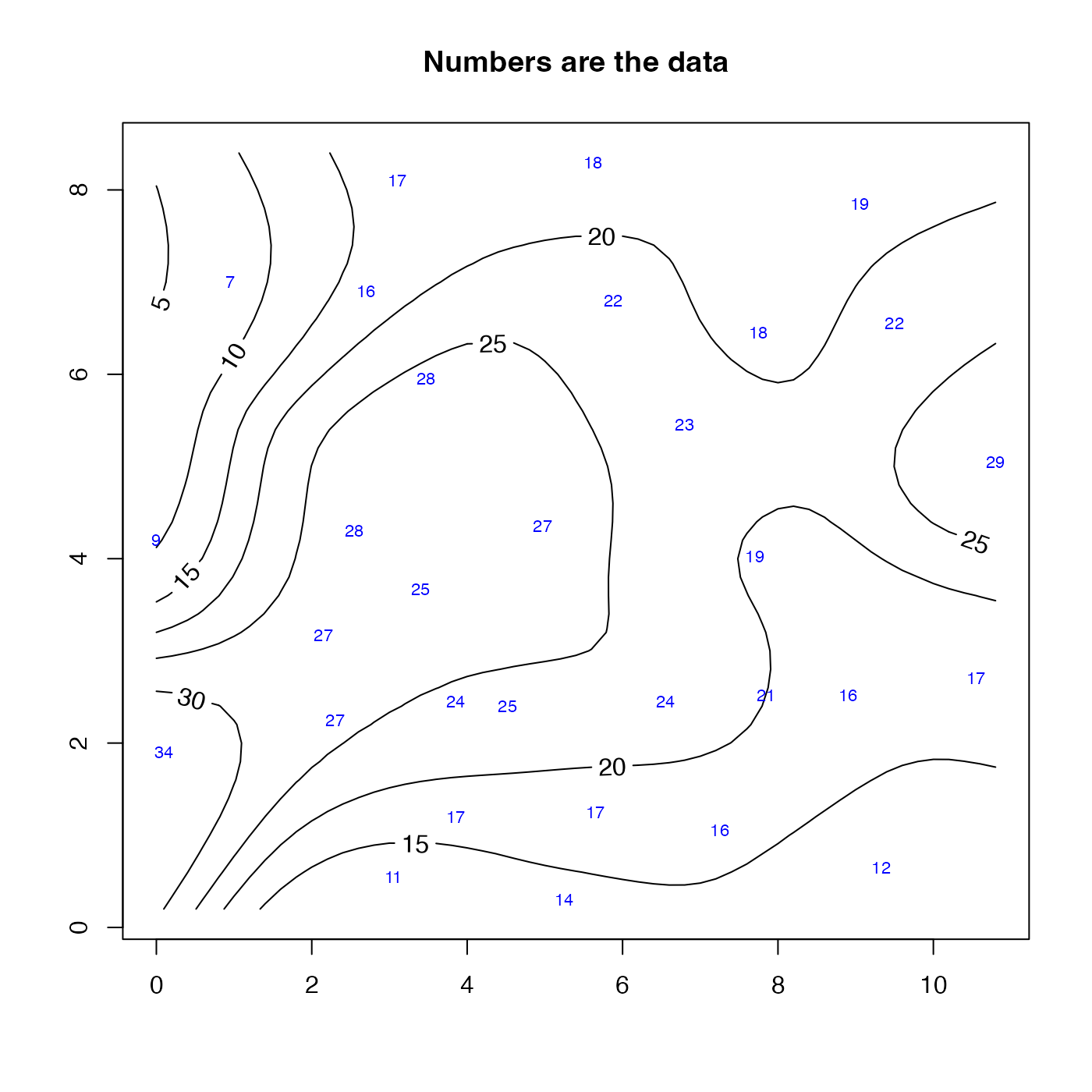
# 1. contouring example, with wind-speed data from Koch et al. (1983)
data(wind)
u <- interpBarnes(wind$x, wind$y, wind$z)
contour(u$xg, u$yg, u$zg, labcex = 1)
text(wind$x, wind$y, wind$z, cex = 0.7, col = "blue")
title("Numbers are the data")


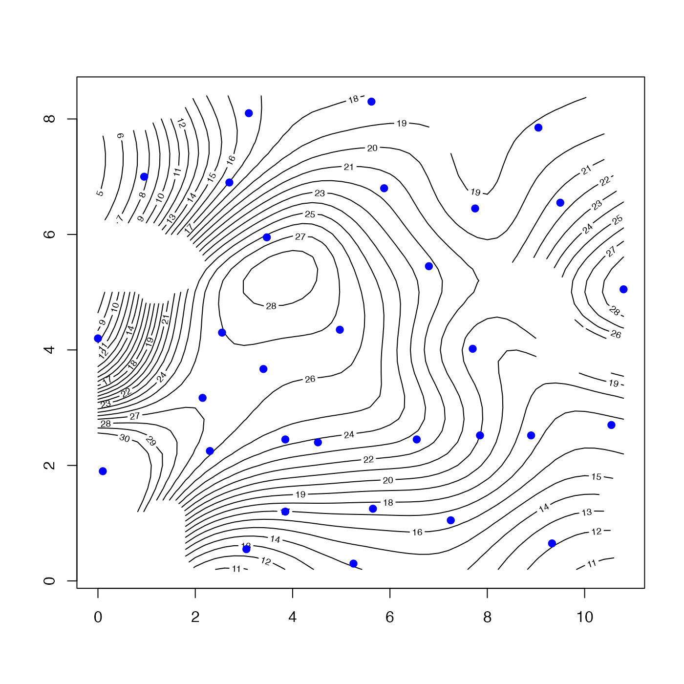
# 2. As 1, but blank out spots where data are sparse
u <- interpBarnes(wind$x, wind$y, wind$z, trim = 0.1)
contour(u$xg, u$yg, u$zg, level = seq(0, 30, 1))
points(wind$x, wind$y, cex = 1.5, pch = 20, col = "blue")


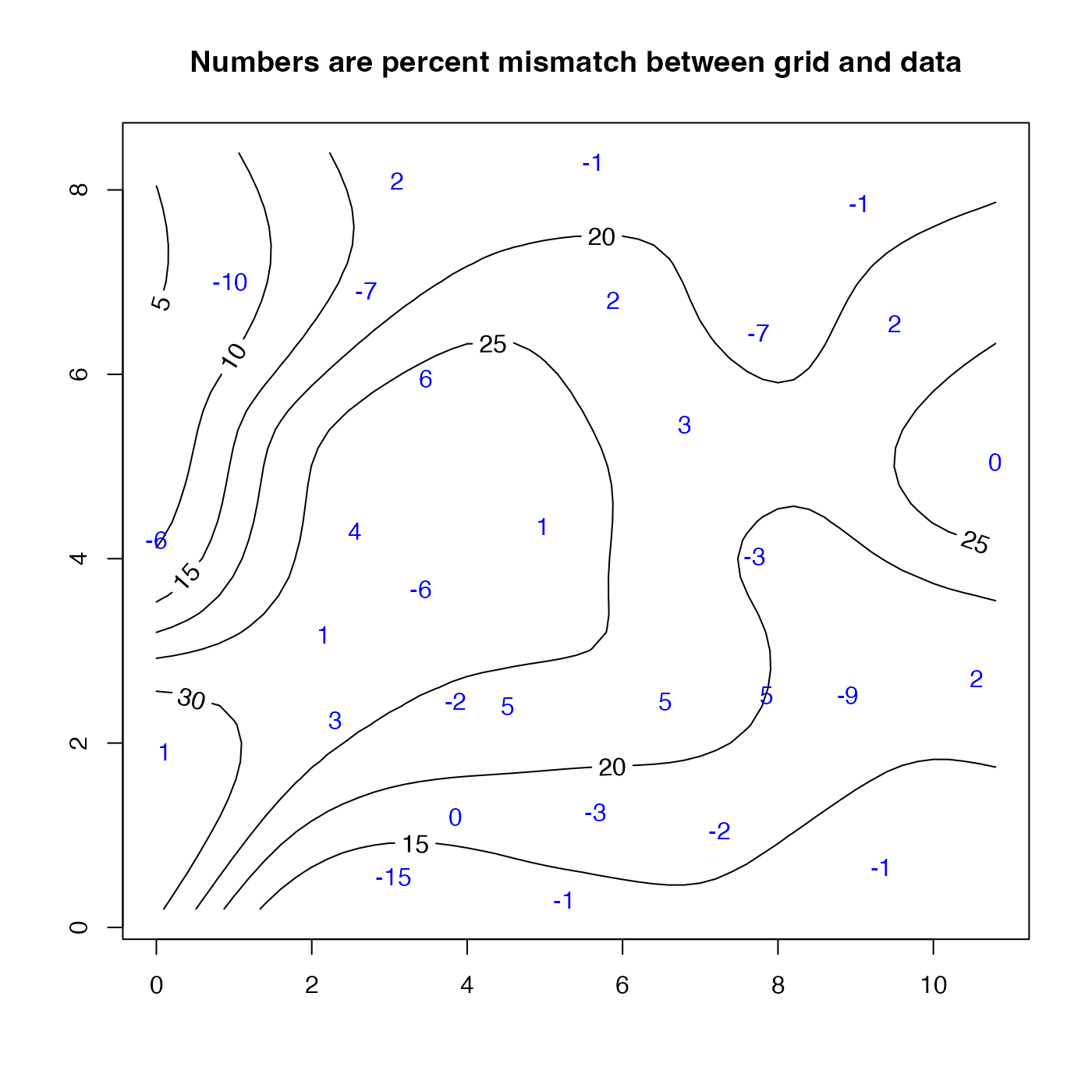
# 3. As 1, but interpolate back to points, and display the percent mismatch
u <- interpBarnes(wind$x, wind$y, wind$z)
contour(u$xg, u$yg, u$zg, labcex = 1)
mismatch <- 100 * (wind$z - u$zd) / wind$z
text(wind$x, wind$y, round(mismatch), col = "blue")
title("Numbers are percent mismatch between grid and data")


# 4. As 3, but contour the mismatch
mismatchGrid <- interpBarnes(wind$x, wind$y, mismatch)
contour(mismatchGrid$xg, mismatchGrid$yg, mismatchGrid$zg, labcex = 1)


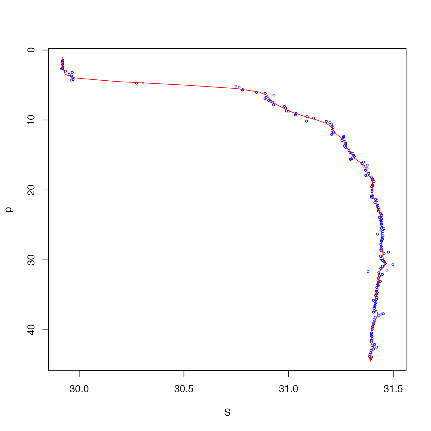
# 5. One-dimensional example, smoothing a salinity profile
data(ctd)
p <- ctd[["pressure"]]
y <- rep(1, length(p)) # fake y data, with arbitrary value
S <- ctd[["salinity"]]
pg <- pretty(p, n = 100)
g <- interpBarnes(p, y, S, xg = pg, xr = 1)
plot(S, p, cex = 0.5, col = "blue", ylim = rev(range(p)))
lines(g$zg, g$xg, col = "red")