Simulate the collision of a ship and a whale

Newtonian mechanics are used, taking the ship as non-deformable, and the whale as being cushioned by a skin layer and a blubber layer. The forces are calculated by shipWaterForce(), whaleSkinForce(), whaleCompressionForce(), and whaleWaterForce() and the integration is carried out with deSolve::lsoda().

Usage

strike(t, state, parms, debug = 0)

Arguments

t: a suggested vector of times (s) at which the simulated state will be reported. This is only a suggestion, however, because strike is set up to detect high accelerations caused by bone compression, and may set a finer reporting interval, if such accelerations are detected. The detection is based on thickness of compressed blubber and sublayer; if either gets below 1 percent of the initial(uncompressed) value, then a trial time grid is computed, with 20 points during the timescale for bone compression, calculated as \(0.5*sqrt(Ly*Lz*a[4]*b[4]/(l[4]*mw)\), with terms as discussed in the documentation for parameters(). If this trial grid is finer than the grid in the t parameter, then the simulation is redone using the new grid. Note that this means that the output will be finer, so code should not rely on the output time grid being
state: A list or named vector holding the initial state of the model: ship position xs (m), ship speed vs (m/s), whale position xw (m), and whale speed vw (m/s).
parms: A named list holding model parameters, created by parameters().
debug: Integer indicating debugging level, 0 for quiet operation and higher values for more verbose monitoring of progress through the function.

Value

strike returns an object of class "strike", which is a list holding 13 items. Nine of these items are time-series vectors, namely time t, ship position xs, ship speed vs, whale position xw, whale speed vw, ship acceleration dvsdt, whale acceleration dvwdt, drag force on the ship SWF, and drag force on the whale WWF. In addition to these time-series items, there are 3 items that are lists: WSF holds time-series of surface forces on the whale; WCF holds time-series of compressive forces on the whale; and parameters holds parameters of the simulation (see parameters() for more information). Finally, there is a logical value named refinedGrid that indicates whether the simulation required a restart because the initial timestep proved inadequate to track the high forces that may arise quickly if bone starts to be compressed appreciably. All quantities are in SI units, s for time, m/s for speed, m/s^2 for acceleration, N for force, etc.

References

See whalestrike() for a list of references.

Author

Dan Kelley

Examples

library(whalestrike)
# Example 1: three plots, as in the default three panels of app()
t <- seq(0, 0.7, length.out = 200)
state <- list(xs = -2, vs = knot2mps(10), xw = 0, vw = 0) # ship speed 10 knots
parms <- parameters()
sol <- strike(t, state, parms)
plot(sol)




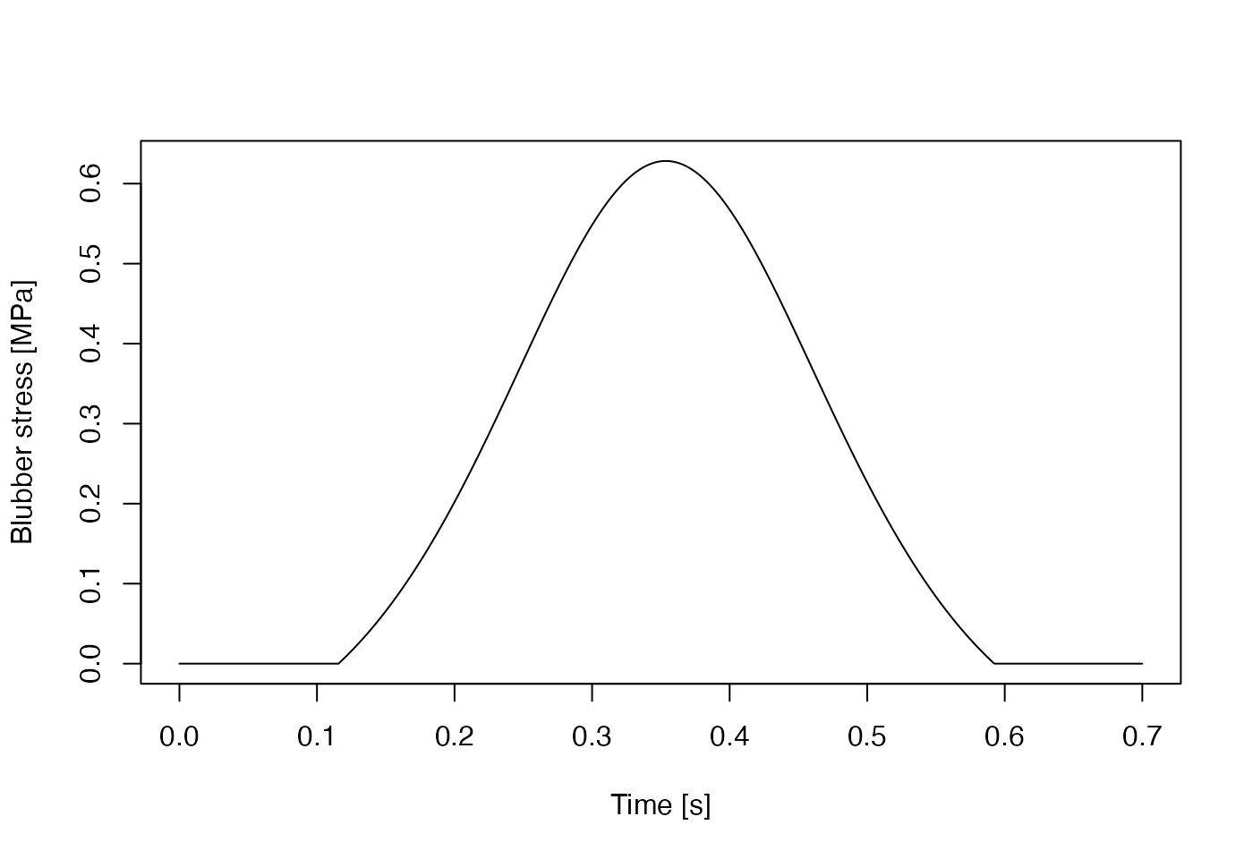
# Example 2: time-series plots of blubber stress and stress/strength,
# for a 200 tonne ship moving at 10 knots
t <- seq(0, 0.7, length.out = 1000)
state <- list(xs = -2, vs = knot2mps(10), xw = 0, vw = 0) # ship 10 knots
parms <- parameters(ms = 200 * 1000) # 1 metric tonne is 1000 kg
sol <- strike(t, state, parms)
plot(t, sol$WCF$stress / 1e6,
    type = "l",
    xlab = "Time [s]", ylab = "Blubber stress [MPa]"
)

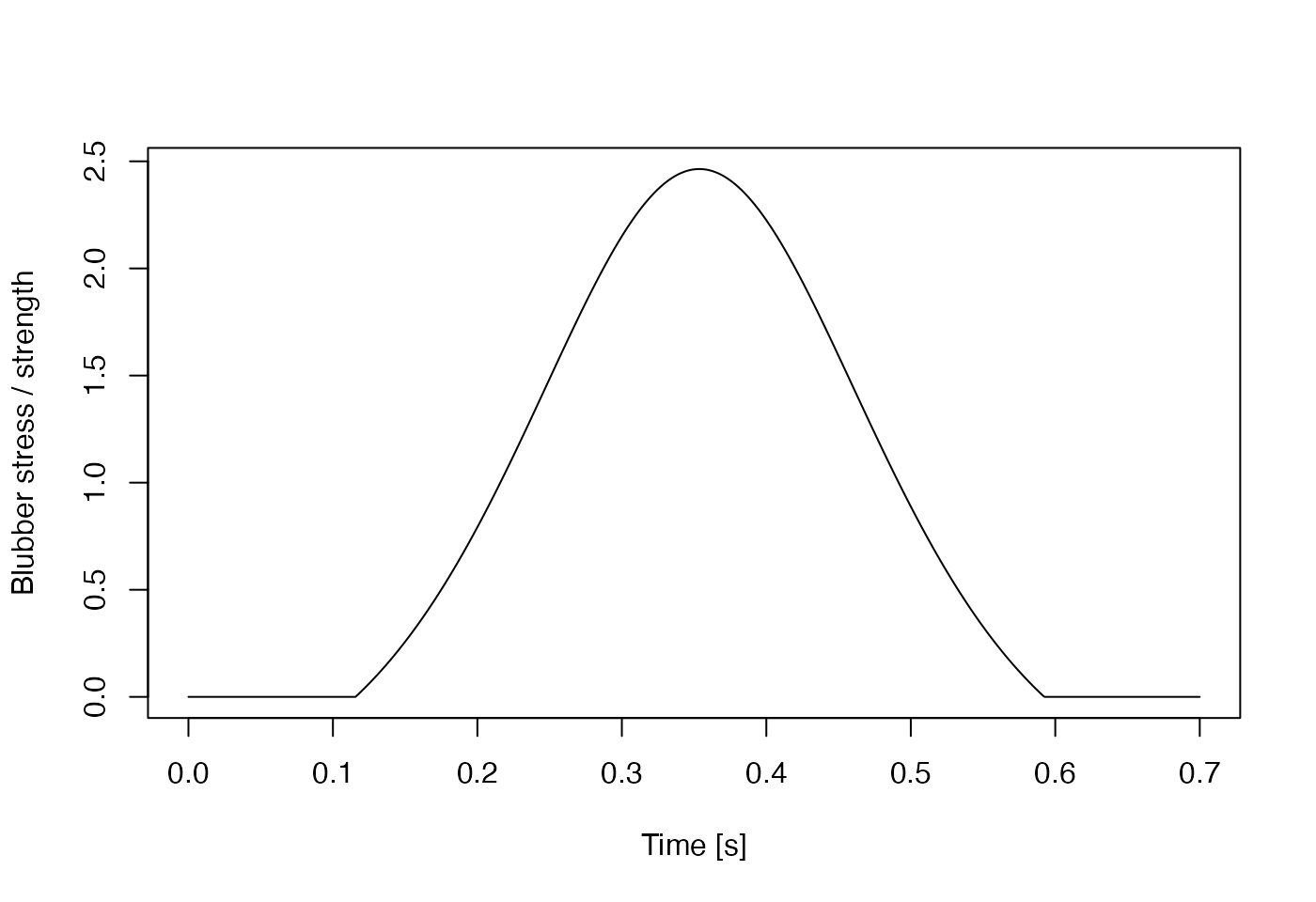
plot(t, sol$WCF$stress / sol$parms$s[2],
    type = "l",
    xlab = "Time [s]", ylab = "Blubber stress / strength"
)


# Example 3: max stress and stress/strength, for a 200 tonne ship
# moving at various speeds.
knots <- seq(0, 10, 1)
maxStress <- NULL
maxStressOverStrength <- NULL
for (speed in knot2mps(knots)) {
    t <- seq(0, 10, length.out = 1000)
    state <- list(xs = -2, vs = speed, xw = 0, vw = 0)
    parms <- parameters(ms = 200 * 1000) # 1 metric tonne is 1000 kg
    sol <- strike(t, state, parms)
    maxStress <- c(maxStress, max(sol$WCF$stress))
    maxStressOverStrength <- c(maxStressOverStrength, max(sol$WCF$stress / sol$parms$s[2]))
}
nonzero <- maxStress > 0
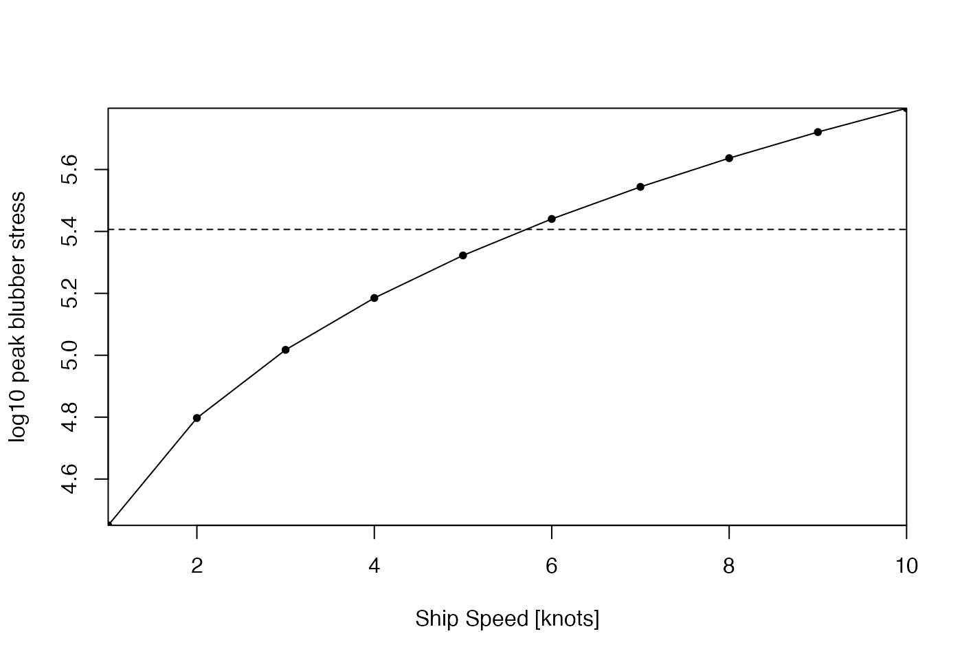
plot(knots[nonzero], log10(maxStress[nonzero]),
    type = "o", pch = 20, xaxs = "i", yaxs = "i",
    xlab = "Ship Speed [knots]", ylab = "log10 peak blubber stress"
)
abline(h = log10(sol$parms$s[2]), lty = 2)

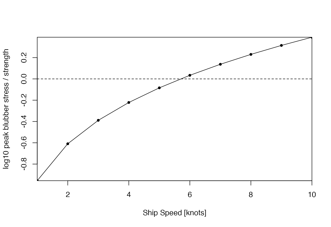
plot(knots[nonzero], log10(maxStressOverStrength[nonzero]),
    type = "o", pch = 20, xaxs = "i", yaxs = "i",
    xlab = "Ship Speed [knots]", ylab = "log10 peak blubber stress / strength"
)
abline(h = 0, lty = 2)