Hodograph of Updated CO2 Dataset
Introduction
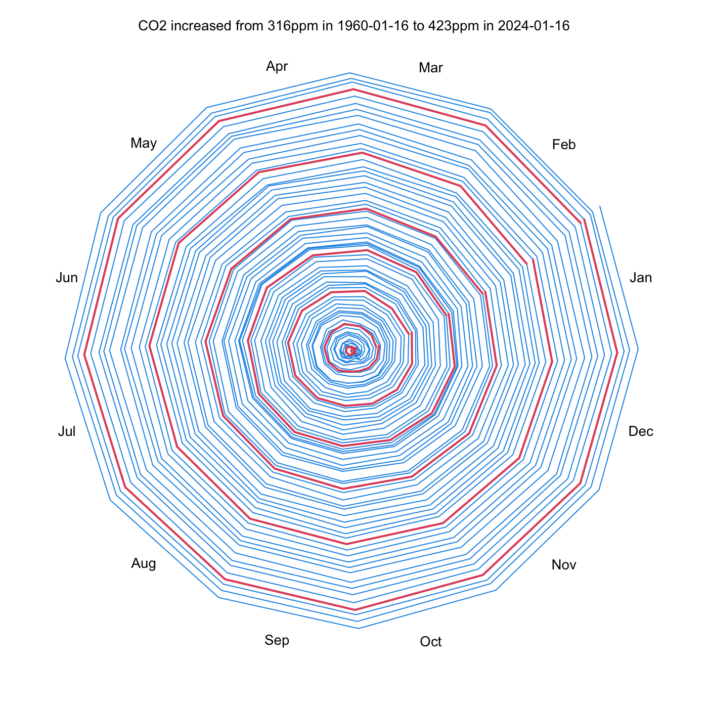
This builds on a previous blog post (reference 1) and uses up-to-date CO2 data (reference 2), plus some changes to the plot, e.g removal of the grid lines and addition of red lines that denote the starts of the decades.
Results
The diagram below show the increasing CO2 signal over the past 64 years. The distance from the centre is proportional to the increase from the initial atmospheric CO2 concentration in value in 1960. The line segments join the monthly values of the dataset. Red lines are used to indicate the first year of each decade.
The general outward spiraling results from an overall trend of increasing CO2 concentration over time. Interannual variability can can also be seen here, as a variation in the spacing of the “rings” of the spiral.
References
-
Posting on 2014-02-08 about making a hodography with the built-in
co2dataset. -
Posting on 2024-02-19 about the up-to-date CO2 dataset, and its comparison with R’s built-in
co2dataset, during the time when they overlap.
Appendix: R code
# Get up-to-date CO2 data
png("2024-02-20-co2-hodograph.png", unit = "in", width = 7, height = 7, pointsize = 10, res = 200)
url <-
    "https://scrippsco2.ucsd.edu/assets/data/atmospheric/stations/in_situ_co2/monthly/monthly_in_situ_co2_mlo.csv"
file <- gsub(".*/", "", url)
message("downloading \"", file, "\" from \"", url, "\"")
download.file(url, file)
lines <- readLines(file)
comment <- grepl("^\"", lines)
dataNames <- read.csv(text = lines[!comment][1])
lines <- lines[!comment]
data <- read.csv(text = lines, skip = 3)
year <- data[, 1] - 1 / 24 + data[, 2] / 12
co2 <- data[, 5]
ok <- co2 > 0
# file has -99.9 values for missing
year <- year[ok]
co2 <- co2[ok]
o <- order(year)
year <- year[o]
co2 <- co2[o]
# just a few intermittent samples prior to 1960
ok <- year >= 1960
year <- year[ok]
co2 <- co2[ok]

png("new-co2-%d.png", unit = "in", width = 7, height = 6, res = 200)
hodograph <- function(x, t, rings, ringlabels = FALSE, axes = FALSE, highlight = NULL, ...) {
    t <- as.POSIXlt(t)
    start <- ISOdatetime(1900 + as.POSIXlt(t[1])$year, 1, 1, 0, 0, 0,
        tz = attr(t, "tzone")
    )
    day <- as.numeric(julian(t, origin = start))
    xx <- x * cos(day / 365 * 2 * pi)
    yy <- x * sin(day / 365 * 2 * pi)
    # axes
    if (missing(rings)) {
        rings <- pretty(sqrt(xx^2 + yy^2))
    }
    rscale <- max(rings)
    theta <- seq(0, 2 * pi, length.out = 200)
    plot(xx, yy,
        asp = 1, xlim = rscale * c(-1.04, 1.04), ylim = rscale * c(-1.04, 1.04),
        type = "n", xlab = "", ylab = "", axes = FALSE
    )
    # month lines
    month <- c("Jan", "Feb", "Mar", "Apr", "May", "Jun", "Jul", "Aug", "Sep", "Oct", "Nov", "Dec")
    day <- c(31, 28, 31, 30, 31, 30, 31, 31, 30, 31, 30, 31)
    rscale <- max(rings)
    for (m in 1:12) {
        # boundaries are for non leap years
        phi <- 2 * pi * (sum(day[1:m]) - day[1]) / sum(day)
        if (axes) {
            lines(rscale * 1.1 * cos(phi) * c(0, 1),
                rscale * 1.1 * sin(phi) * c(0, 1),
                col = "darkgray"
            )
        }
        phi <- 2 * pi * (0.5 / 12 + (m - 1) / 12)
        text(1.1 * rscale * cos(phi), 1.1 * rscale * sin(phi), month[m])
        if (axes) {
            for (r in rings) {
                if (r > 0) {
                    gx <- r * cos(theta)
                    gy <- r * sin(theta)
                    lines(gx, gy, col = 2)
                    if (ringlabels) {
                        text(gx[1], 0, format(r))
                    }
                }
            }
        }
    }
    lines(xx, yy, ...)
    for (h in highlight) {
        tstart <- ISOdatetime(h, 1, 1, 1, 0, 0, tz = "UTC")
        tstop <- ISOdatetime(h + 1, 2, 1, 0, 0, 0, tz = "UTC")
        look <- tstart <= t & t <= tstop
        lines(xx[look], yy[look], col = 2, lwd = 2)
    }
}
t0 <- ISOdatetime(1959, 1, 1, 0, 0, 0, tz = "UTC")
t <- t0 + (year - 1959) * 365.25 * 86400
par(mar = rep(3, 4))
co2start <- head(co2, 1)
hodograph(
    x = co2 - co2start, t = t, rings = seq(0, 100, 10), col = 4,
    #highlight = c(1974, 1993, 1998)
    highlight = seq(1960, 2024, 10)
)
label <- sprintf(
    "CO2 increased from %.0fppm in %s to %.0fppm in %s",
    co2[1],
    format(t[1], "%Y-%m-%d"),
    tail(co2, 1),
    format(tail(t, 1), "%Y-%m-%d")
)
mtext(label, line = 1)