Bathymetry and Topography near Nova Scotia
This is a followup to two previous posts (here and here), dealing with representing the shape of the earth surface with a shaded scheme. Here I discuss a view of land/sea topography in the region of Nova Scotia, Canada.
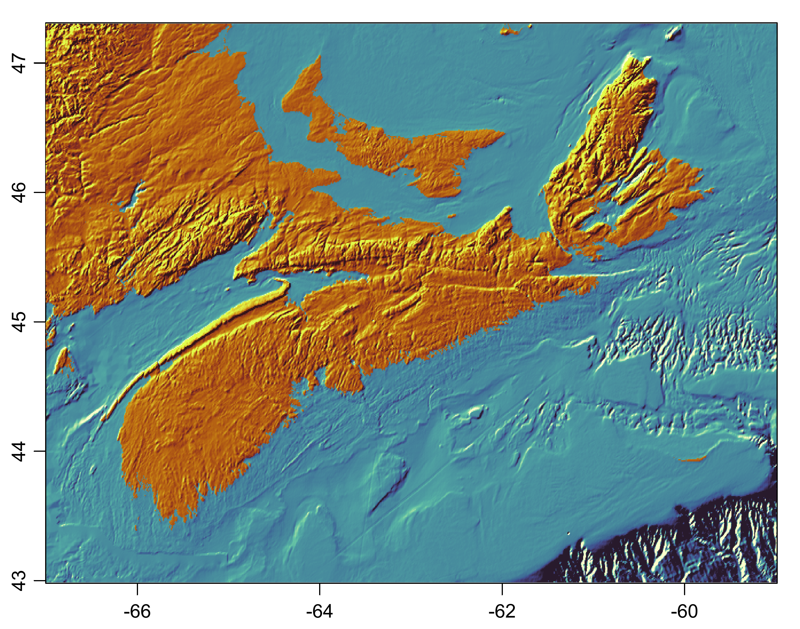
In the diagram shown below, blue hues represent the ocean, and golden hues represent the land. As with the two previous posts, brightness is based on surface slope, meant to evoke illumination by a light source in the upper-left corner, pointing towards the lower-right corner.
There is a lot to see in this diagram. Nova Scotians will likely find their own favourite spots, but I’ll point out just a few.
- The Annapolis Valley, to the south of the Bay of Fundy, is particularly prominent as a flat area bounded by high land to the north and soutrh.
- Cape Breton has a complex pattern of relief that is will be well known to those who have travelled there.
- A fault line running from east to west at about 45.5N is visible both above and below sealevel. The high lands to the north of that line, known as the Cobequid Mountains, are quite visible in this view. For more on this assemblage, and the geology of Nova Scotia generally, see Pe-piper and Piper (2003) and references therein.
References
- George Pe-piper, David J.W. Piper, “A synopsis of the geology of the Cobequid Highlands, Nova Scotia”, Atlantic Geology, 2003 https://journals.lib.unb.ca/index.php/ag/article/view/1259/1652
R code to make the diagram
This code uses two packages, oce and dod. The first is on CRAN, and may be
installed using
install.packages("oce")
while the second is not yet on CRAN, and must be installed with
# install.packages("remotes")
remotes::install_github("dankelley/dod")
where the first line must be un-commented if remotes is not already
installed.
If you use this as a pattern for a diagram of your own, there are two things you will likely want to adjust.
- The
resolutionparameter ofdod.topo(), which is the resolution of the topographic matrix in arc minutes. (One arc minute in latitude corresponds to 1 nautical mile, or a bit under 2 km. See?dod.topofor more on this.) - The
heightparameter ofpng(), which I have adjusted here to remove white bands that otherwise appear at either the top and bottom of the image, or the left and right. These bands occur if the aspect ratio of the axis frame is not equal to the aspect ratio of the data view. A few minutes of adjustment is all it should take to find a good value. Note that I run this code in non-interactive mode. If you tend to run code through RStudio or in another interactive manner, you can adjust the plot size and redraw until the white bands go away, but I recommend working non-interactively (or eliminating theifcondistion) because then your code will be reproducible and you can use the same parameters for other plots. - You may wish to alter the definition of
Q. Try using slightly larger or smaller values (in the range from 0 to 1) to see how that affects the contrast. Your goal will likely be to see lots of detail, without having some areas be overly dark or light. Think of this as a sort of contrast parameter.
Q <- 0.95 # quantile for slope cutoff
library(oce)
library(dod)
topoFile <- dod.topo(-67, -59, 43, 47.3, resolution = 0.5)
topo <- read.topo(topoFile)
x <- topo[["longitude"]]
y <- topo[["latitude"]]
z <- topo[["z"]]
asp <- 1 / cos(mean(y) * pi / 180)

g <- grad(z, x, y)
G0 <- asp * g$gx - g$gy # note the asp factor
zlim <- quantile(abs(G0), Q) * c(-1, 1)
if (!interactive()) {
    png("topobathy_NS.png",
        width = 7, height = 5.5, unit = "in", res = 400,
        type = "cairo", antialias = "none", family = "Arial"
    )
}
# Water
water <- G0
water[z > 0] <- NA
cmwater <- colormap(
    zlim = zlim,
    col = cmocean::cmocean("deep", direction = -1)
)
imagep(x, y, water,
    asp = asp,
    colormap = cmwater,
    decimate = FALSE,
    mar = c(2.0, 2.0, 1.0, 1.0),
    drawPalette = FALSE
)
# Land
land <- G0
land[z < 0] <- NA
cmland <- colormap(zlim = zlim, col = cmocean::cmocean("solar"))
imagep(x, y, land,
    asp = asp,
    colormap = cmland,
    decimate = FALSE,
    add = TRUE,
    drawPalette = FALSE
)
if (!interactive()) {
    dev.off()
}