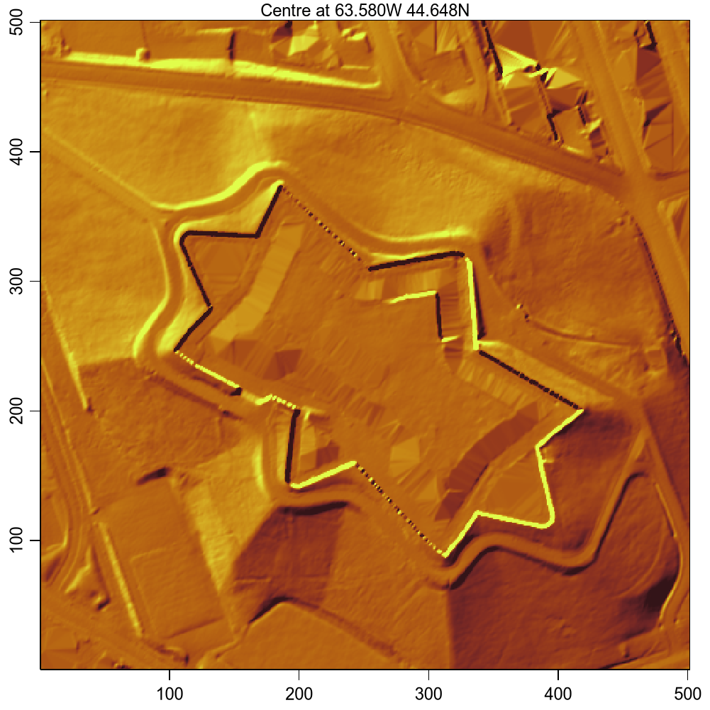
Lidar image for Citadel Hill in Halifax NS
I learned recently that LIDAR-based topographic elevation data are available for many spots in Nova Scotia (see Reference 1), so I downloaded a dataset that holds such data and wrote R code to examine some spots of interest. Reference 2, a video, shows an initial exploration of Point Pleasant Park. In this blog posting, I focus on something that will be more familiar to the public: the Citadel.
I’ll let the code speak for itself. Examination of the image reveals that sometimes the LIDAR data show what looks to be triangular interpolation, presumably across data that are questionable. I think there is also a mechanism to “see through” some features, e.g. trees, but I do not know much about that. What I do know is that land features are very clearly visible. The Citadel provides an example that I hope interests readers.
A few things are worth noting:
- For this particular centre point,
L(the image extent) cannot be made much larger than 600 (metres), because that will extend beyond the limits of the dataset. I could code to handle that, of course, but haven’t bothered here. I have not thought about how to stitch together adjacent datasets. - The colour scheme being used here is just one of many that users might try.
In addition to the R standards, the schemes provided by the
cmoceanpackage (Reference 3) are paricularly worth exploring. - There is no water present in this view, so no blue appears. Obviously, if a
colour scheme containing blue were to be used, the missing-value colour
would have to be changed from
"blue"as used here. - Reference 4 is a somewhat dated, but useful, video about how LIDAR works. I think there is a typo on a slide about accuracy, stating that the unit was centimetre, but I think it is metre. Still, the talk is very clear, and at a level that suits the discussion here.
# Data source
#     https://nsgi.novascotia.ca/datalocator/elevation/

# Part 1: things to edit
dir <- "~/Downloads/1044600063500_201901_DEM"
name <- "citadel"
L <- 500 # extent in m (cannot be much larger since at image edge)
centre <- data.frame(ID = 1, X = -63.5804, Y = 44.6475)
Q <- 0.99

# Part 2: things that likely do not need editing
width <- 7
height <- 7
res <- round(2 * L / width)
library(raster) # to read image
library(oce) # for imagep
library(sf) # for coordinate calculations

# Load data
l <- list.files(dir, "*tif$", full.names = TRUE) |> raster()
getLidarMatrix <- function(l) {
    rval <- getValues(l, format = "matrix") |> t()
    rval[, dim(rval)[2] |> seq_len() |> rev()]
}
h <- getLidarMatrix(l)

# Set a focus region (square)
projection <- l@srs
coordinates(centre) <- c("X", "Y")
proj4string(centre) <- CRS("+proj=longlat +datum=WGS84")
C <- spTransform(centre, CRS(projection))
C <- c(xmin(C) - xmin(l), ymin(C) - ymin(l))
pin <- function(x) {
    # FIXME: should also check if too large
    x <- as.integer(x)
    ifelse(x < 1, 1, x)
}
look <- pin(c(C[1] - L / 2, C[1] + L / 2, C[2] - L / 2, C[2] + L / 2))
H <- h[look[1]:look[2], look[3]:look[4]]
dimH <- dim(H)
x <- seq_len(dimH[1]) # metres
y <- seq_len(dimH[2])
g <- oce::grad(H, x, y)
G <- g$gx - g$gy # FIXME: allow for illumination azimuth and altitude
water <- H <= 0
q <- as.numeric(quantile(G[!water], Q))
GG <- G
GG[water] <- NA

if (!interactive()) {
    png(paste0("lidar_", name, ".png"),
        width = width, height = height, unit = "in", res = res,
        type = "cairo", antialias = "none", family = "Arial"
    )
}
imagep(x, y, GG,
    zlim = c(-q, q),
    asp = 1,
    col = cmocean::cmocean("solar"), # golden hues
    decimate = FALSE,
    missingColor = "blue", # water
    mar = c(2.0, 2.0, 1.0, 1.0),
    drawPalette = FALSE
)
mtext(sprintf("Centre at %.3fW %.3fN", -centre$X, centre$Y))
if (!interactive()) {
    dev.off()
}
message("Created ", paste0("lidar_", name, ".png"))
References and resources
-
Source of LIDAR images for Nova Scotia https://nsgi.novascotia.ca/datalocator/elevation
-
Youtube video about a LIDAR image of Point Pleasant Park in Halifax, Nova Scotia, with some notes on how it compares with google imagery. https://www.youtube.com/watch?v=hvkb3fsms6g
-
The
cmoceanpackage for colour schemes. https://cran.r-project.org/web/packages/cmocean/vignettes/cmocean.html -
Youtube video about LIDAR methodology. https://www.youtube.com/watch?v=PRE5KV2_w3Q