Draw polygon between two xy curves

This adds to an existing plot by filling the area between the lower=lower(x) and upper=upper(x) curves. In most cases, as shown in “Examples”, it is helpful to use xaxs="i" in the preceding plot call, so that the polygon reaches to the edge of the plot area.

fillplot(x, lower, upper, ...)

Arguments

x

Coordinate along horizontal axis

lower

Coordinates of the lower curve, of same length as x, or a single value that gets repeated to the length of x.

upper

Coordinates of the upper curve, or a single value that gets repeated to the length of x.

...

passed to polygon(). In most cases, this will contain col, the fill colour, and possibly border, the border colour, although cross-hatching with density and angle is also a good choice.

Author

Dan Kelley

Examples

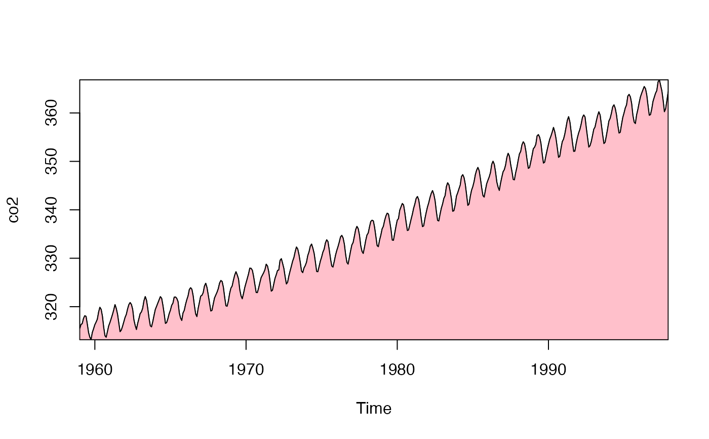
# 1. CO2 record
plot(co2, xaxs = "i", yaxs = "i")
fillplot(time(co2), min(co2), co2, col = "pink")


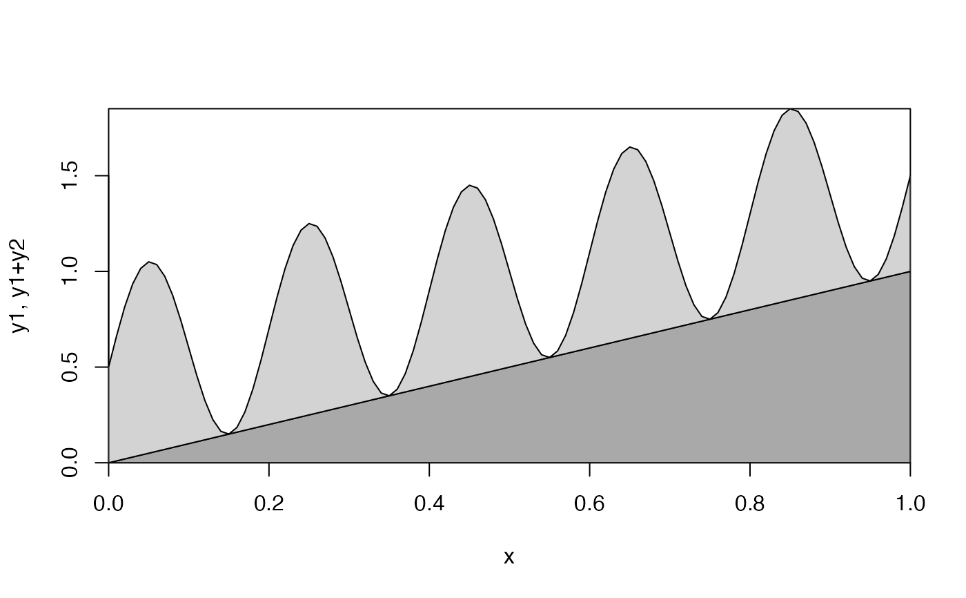
# 2. stack (summed y) plot
x <- seq(0, 1, 0.01)
lower <- x
upper <- 0.5 * (1 + sin(2 * pi * x / 0.2))
plot(range(x), range(lower, lower + upper),
    type = "n",
    xlab = "x", ylab = "y1, y1+y2",
    xaxs = "i", yaxs = "i"
)
fillplot(x, min(lower), lower, col = "darkgray")
fillplot(x, lower, lower + upper, col = "lightgray")