If saveFile is TRUE, then the file is saved for later use. Its
first line will be a header. A column named "Date" may be decoded
into a POSIX time value using lubridate::ymd_hms().
Arguments
- id
character value indicating the ID of the desired station. This may be discovered by using
dod.river.index()first. This defaults to"01EJ001", for the Sackville River at Bedford.- region
character value indicating the province or territory in which the river gauge is sited. This defaults to
"NS.- interval
character value, either
"daily"or `"hourly", indicating the time interval desired. (The first seems to yield data in the current month, and the second seems to yield data since over the last 1 or 2 days.)- saveFile
logical value indicating whether to save the file for later use. This can be handy because the server does provide archived data. The filename will be as on the server, but with the main part of the filename ending with a timestamp. This file name is printed during processing, and it may be read later with
read.csv(), with its time column being decoded withlubridate::ymd_hms(); perhaps the server has information on the meanings of the other columns, or perhaps you will be able to guess.- debug
integer indicating the level of debugging information that is printed during processing. The default,
debug=0, means to work quietly.
Value
a data frame containing the data, with columns named "time" and
"level" (m), "grade" and "discharge" (m^3/s). (Note that files contain
other columns; if you want them, save the file and read it
as explained in ‘Details’.)
References
Gore, James A., and James Banning. “Chapter 3 - Discharge Measurements and Streamflow Analysis.” In Methods in Stream Ecology, Volume 1 (Third Edition), edited by F. Richard Hauer and Gary A. Lamberti, 49–70. Boston: Academic Press, 2017. https://doi.org/10.1016/B978-0-12-416558-8.00003-2.
Examples
library(oce)
#> Loading required package: gsw
library(dod)
dir <- dod.river.index() # defaults to Sackville River at Bedford
data <- dod.river(id = dir$id)
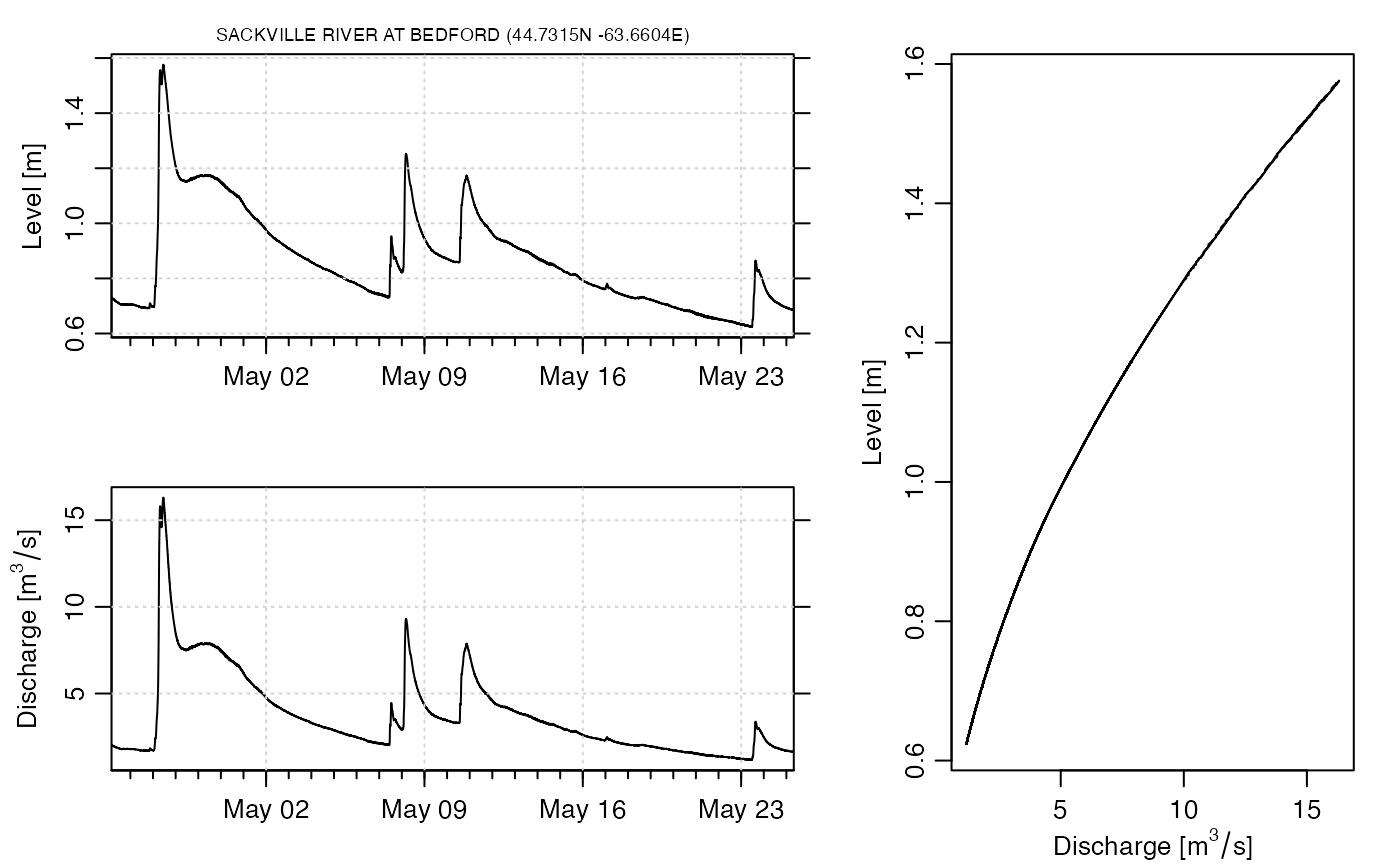
# Plot a 3-panel summary graph; see e.g. Gore and Banning (2017) for more
# information on discharge.
layout(matrix(c(1, 3, 2, 3), 2, 2, byrow = TRUE), width = c(0.6, 0.4))
oce.plot.ts(data$time, data$level,
xaxs = "i",
xlab = "", ylab = "Level [m]",
drawTimeRange = FALSE, grid = TRUE
)
mtext(sprintf("%s (%.4fN %.4fE)", dir$name, dir$latitude, dir$longitude),
line = 0.2, cex = 0.7 * par("cex")
)
oce.plot.ts(data$time, data$discharge,
xaxs = "i",
xlab = "", ylab = expression("Discharge [" * m^3 / s * "]"),
drawTimeRange = FALSE, grid = TRUE
)
plot(data$discharge, data$level,
type = "l",
xlab = expression("Discharge [" * m^3 / s * "]"), ylab = "Level [m]"
)