Introduction to the atm Package
Dan Kelley (https://orcid.org/0000-0001-7808-5911)
2025-08-27
Source:vignettes/atm.Rmd
atm.RmdAbstract. This shows how to plot a recent atmospheric sounding at the default location, Shearwater, Nova Scotia, Canada.
Plot a sample sounding for Shearwater, Nova Scotia, Canada.
This example uses a sample data file that is provided in the package, because otherwise building the vignette can yield an error, if the server (Reference 1) is unreachable or is too busy to return files.
There are several errors and deficiencies with this graph, including the following.
- water fraction should be added
- perhaps text summaries should be added, although I’m not sure on this because the summaries in the data files don’t have things that seem most interesting, like CAPE
library(atm)
#> Loading required package: S7
file <- system.file("extdata", "Shearwater_2024-07-11.txt.gz", package = "atm")
sounding <- readSounding(file)
plot(sounding)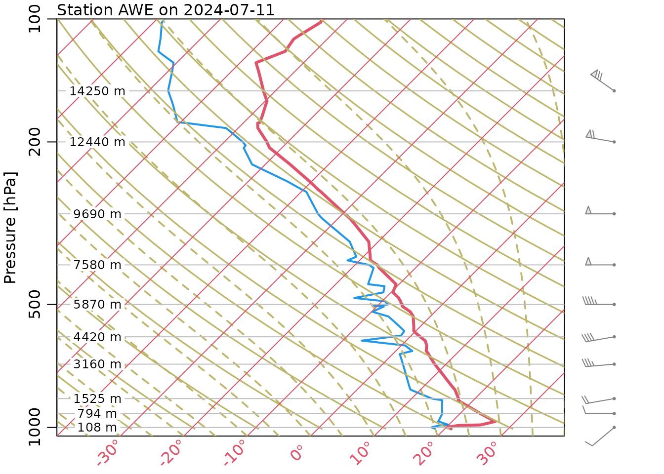
Skew-T log-P sounding profile at Shearwater, Nova Scotia, Canada, on July 11, 2024. The red line represents temperature and the slighly thinner blue line represents dew point. The solid dark green curves are dry adiabats, and the dashed ones are moist adiabats (think of dash as representing rain). All of these curves are skewed, so that to read values, find one of the red 45 degree lines and trace it down to a temperature on the bottom axis.