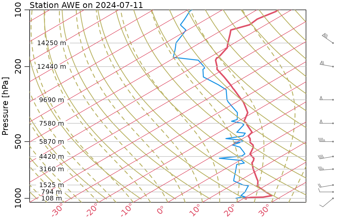
Display sounding data in profile form. Red lines sloping from bottom-left to top-right indicate temperatures. The thicker red curve is in-situ temperature. The thinner blue curve is dew-point temperature. The curved olive green lines indicate wet and dry adiabats, with dashed lines used for the former. The vertical axis represents pressure, and thin horizontal lines are drawn to indicate standard heights. The wind barbs drawn to the right of the profile indicate velocities at those heights in meteorological convention for speeds in knots.
Arguments
- sounding
the result of a call to
readSounding().- item
character value indicating what to plot. At the moment, the only choices is the default,
"DWPT+TEMP".- legend
logical value indicating whether to show a legend in the top- left corner. This is FALSE by default.
- mar
4-element numeric vector specifying margins, in the standard way (i.e. this is handed to
par()by this function). The default is set to give space for height indications in the right margin.- mgp
3-element numeric vector specifying axis spacing, in the usual way (i.e. this is handed to
par()by this function). The default removes some whitespace in the margins.- debug
an integer specifying whether information is to be printed during processing. The default, 0, means to avoid such printing. Any positive value means to print some information. (That information will vary over the course of evolution of the code, so do not rely on particular behaviour.)
References
https://www.noaa.gov/jetstream/upperair/skew-t-log-p-diagramsVisual Explanation of Meteorological Skew T Log P Sounding Diagrams, 2019. https://www.youtube.com/watch?v=7p7c85hhgOo.
Examples
library(atm)
# Normally, would download the file with downloadSounding()
file <- system.file("extdata", "Shearwater_2024-07-11.txt.gz", package = "atm")
sounding <- readSounding(file)
plot(sounding)