This posting shows how one might perform demodulation in R. It is assumed that readers are generally familiar tith the procedure.
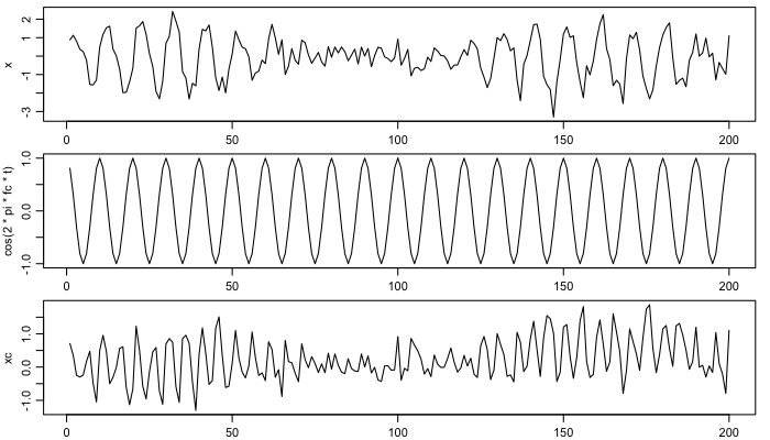
First, create some fake data, a carrier signal with period 10, modulated over a long timescale, and with phase drifting linearly over time.
1
2
3
4
5
6
7
8
9
10
period <- 10
fc <- 1 / period
fs <- 1
n <- 200
t <- 1:n
AMP <- 1 + sin(0.5 * fc * t)
PH  <- 50 * t / max(t)
noise <- rnorm(n, sd=0.5)
signal <- AMP * sin(2 * pi * fc * t + PH*pi/180)
x <- signal + noise
Next, create the base sine and cosine time-series, varying with the known frequency, and plot these.
1
2
3
4
5
6
xc <- x * cos(2 * pi * fc * t)
xs <- x * sin(2 * pi * fc * t)
par(mar=c(1.75,3,1/2,1), mgp=c(2, 0.7, 0), mfcol=c(3,1))
plot(t, x, type='l')
plot(t, cos(2 * pi * fc * t), type='l')
plot(t, xc, type='l')

Smooth the results, and infer amplitude and phase. Here, the butterworth filter parameters are smoothing more than in the Matlab demod() function (reference 1).
1
2
3
4
5
6
7
8
w <- 2 * fc / fs
## Here, we use more smoothing
w <- w / 5
filter <- signal::butter(5, w)    # FIXME: why extras on w?
xcs <- signal::filtfilt(filter, xc)
xss <- signal::filtfilt(filter, xs)
amp <- 2 * sqrt(xcs^2 + xss^2)
phase <- 180 / pi * atan2(xcs, xss)
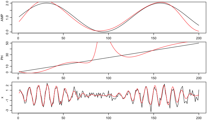
Finally, show the amplitude and phase (black for supplied, red for inferred), as well as the original time series (again, black) and the reconstructed signal (red).
1
2
3
4
5
6
7
8
par(mar=c(1.75,3,1/2,1), mgp=c(2, 0.7, 0), mfcol=c(3,1))
plot(t, AMP, type='l')
lines(t, amp, col='red')

plot(t, PH, type='l')
lines(t, phase, col='red')
plot(t, x, type='l', pch=20)
lines(t, amp * sin(2 * pi * fc * t + phase*pi/180), col='red')

Note that altering the smoothing properties alters the results somewhat. Here, more smoothing is used than in the matlab code (reference 2). For better results, it may make sense to detrend the data before filtering, as described in a previous blog item.
Resources
-
Source code: 2014-04-17-demodulation.R