Introduction

Smoothing hydrographic profiles with conventional time-series methods is problematic for two reasons: (a) the data are commonly not equi-spaced in depth and (b) the data seldom lack trends in depth. The issues and their solutions are illustrated without much discussion here.

The first step in making the graph shown above is to load the oce library and create a function that measures daylength by finding sunrise and sunset times. Note that uniroot(), which is used to find times of zero solar altitude, needs lower and upper limits on t, and these are calculated by looking back and then forward a half-day. This works well for application to Halifax, but in other timezones other offsets would be needed. Interested readers might want to devised a method based on the longitude, which can be transformed into a timezone.

Methods

The first step is to load the data and extract dependent and independent variables, here S and p.

1
2
3
4
5
library(oce)
library(signal)
data(ctd)
S <- ctd[['salinity']]
p <- ctd[['pressure']]

Next, one must create equispaced data, for filtering to make any sense at all.

1
2
3
dp <- median(diff(p))
pp <- seq(min(p), max(p), dp)
S0 <- approx(p, S, pp)$y

Now comes something that must be established by the actual task at hand: setting the critical frequency for the filter (as a ratio to Nyquist). In this case, a somewhat arbitrary frequency is selected, and then both first-order and second-order filters are created.

1
2
3
W <- dp / 2
f1 <- butter(1, W)
f2 <- butter(2, W)

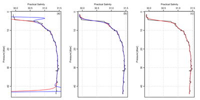
Now, set up for a three-panel plot.

1
par(mfrow=c(1, 3))

For the left-hand panel, show the raw data in black, and the two filters in red and blue.

1
2
3
4
5
6
plotProfile(ctd, xtype="salinity", type='l')
S0f1 <- filtfilt(f1, S0)
S0f2 <- filtfilt(f2, S0)
lines(S0f1, pp, col='red')
lines(S0f2, pp, col='blue')
mtext("(a) ", side=3, adj=1, line=-5/4, cex=3/4)

For the middle panel, detrended the profile, and then filter.

1
2
3
4
5
6
7
plotProfile(ctd, xtype="salinity", type='l')
Sd <- detrend(pp, S0)
S1f1 <- filtfilt(f1, Sd$Y) + Sd$a + Sd$b * pp
S1f2 <- filtfilt(f2, Sd$Y) + Sd$a + Sd$b * pp
lines(S1f1, pp, col='red')
lines(S1f2, pp, col='blue')
mtext("(b) ", side=3, adj=1, line=-5/4, cex=3/4)

For the right-hand panel, use a smoothing spline instead of a filter.

1
2
3
4
5
spline <- smooth.spline(pp, S0, df=3/W)
S2 <- predict(spline)$y
plotProfile(ctd, xtype="salinity", type='l')
lines(S2, pp, col='red')
mtext("(c) ", side=3, adj=1, line=-5/4, cex=3/4)

Results

Filtering a non-detrended profile is a generally a bad idea. There is almost always a zero-offset problem, and also most properties vary dramatically with depth, so detrending is required as well as zero offsetting. The advantage of detrending is illustrated in the left-hand and middle panels.

Smoothing splines provide an attractive alternative to filtering, especially in the not-uncommon cases in which derivative are required. However, a disadvantage of splines is that there is no simple way to describe the method to those who are not familiar with them. In some branches of the literature, splines will be understood by readers, and in others, they will be a mystery that will waste a review cycle for the education of referees. There is also a problem in describing the spline simply in terms that have physical meaning. For example, spline smoothness is here controlled by setting the df argument, but this has no simple analogy to physics, as perhaps the half-power frequency of a filter might (in terms of spectral models of finestructure, say).