Motivation

Using R within a latex document can be a component of reproducible research, offering (a) some assurance against typographical errors in transcribing results to the latex file and (b) the ability for others to reproduce the results.

For example, one might like to explain how close the computed integral of the Witch of Agnesi function

1
2
woa <- function(x, a=1) 8 * a^3 / (x^2 + 4*a^2)
integrate(woa, -Inf, Inf)

## 12.56637 with absolute error < 1.3e-09

is to the true value of $4\pi$. One way to do that is to compute the mismatch

1
2
estimate <- integrate(woa, -Inf, Inf)$value
theory <- 4 * pi

and to write something like

\dots the misfit is \Sexpr{abs(estimate-theory)}

in latex. However, the slew of digits is not especially useful, and the computer-type exponential notation is not conventional in written work.

It would be good to have a function that writes such results in latex format.

Methods

A trial function is below.

1
2
3
4
5
6
7
8
9
10
11
12
13
14
15
16
17
18
scinot <- function(x, digits=2, showDollar=FALSE)
{
    sign <- ""
    if (x < 0) {
        sign <- "-"
        x <- -x
    }
    exponent <- floor(log10(x))
    if (exponent) {
        xx <- round(x / 10^exponent, digits=digits)
        e <- paste("\\\\times 10^{", as.integer(exponent), "}", sep="")
    } else {
        xx <- round(x, digits=digits)
        e <- ""
    }
    if (showDollar) paste("$", sign, xx, e, "$", sep="")
    else paste(sign, xx, e, sep="")
}

and a latex/sweave test use is

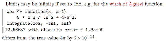
Limits may be infinite if set to \texttt{Inf}, e.g. for the witch of Agnesi
function
<<>>=
woa <- function(x, a=1)
    8 * a^3 / (x^2 + 4*a^2)
integrate(woa, -Inf, Inf)
@
<<results=hide, echo=false>>=
woa <- function(x, a=1)
    8 * a^3 / (x^2 + 4*a^2)
i <- integrate(woa, -Inf, Inf)$value
err <- abs((i - 4 * pi) / (4 * pi))
@
the results differ from the true value $4\pi$ by $\Sexpr{scinot(err, 0)}$.

which yields as shown in the screenshot below. (Note that there is some colourization and margin decoration that is not described by the code given above.)

References and resources

1. R source code used here: 2015-03-22-scinot.R.

2. Jekyll source code for this blog entry: 2015-03-22-scinot.Rmd