Introduction
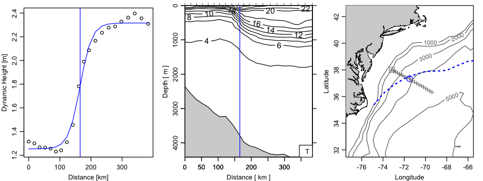
Definitions of Gulf Stream location sometimes centre on thermal signature, but it might make sense to work with dynamic height \(\eta\) instead. This is illustrated here, using a \(\tanh\) model for \(\eta=\eta(x)\), with \(x\) the distance along the transect. The idea is to select \(x_ 0\), the halfway point in the \(\tanh()\) function, where the slope is maximum and where therefore the inferred geostrophic velocity peaks.
Methods and results
1
library(oce)
## Loading required package: methods
## Loading required package: mapproj
## Loading required package: maps
1
2
3
4
5
6
7
8
9
10
11
12
13
14
15
16
17
18
19
20
21
22
23
24
25
26
27
28
29
30
31
32
33
34
35
36
37
38
39
40
41
data(section)
## Extract Gulf Stream (and reverse station order)
GS <- subset(section, 109<=stationId & stationId<=129)
GS <- sectionSort(GS, by="longitude")
GS <- sectionGrid(GS)
## Compute and plot normalized dynamic height
dh <- swDynamicHeight(GS)
h <- dh$height
x <- dh$distance
par(mfrow=c(1, 3), mar=c(3, 3, 1, 1), mgp=c(2, 0.7, 0))
plot(x, h, xlab="Distance [km]", ylab="Dynamic Height [m]")
## Fit to tanh, with x0 line
m <- nls(h~a+b*(1+tanh((x-x0)/L)), start=list(a=0,b=1,x0=100,L=100))
hp <- predict(m)
lines(x, hp, col='blue')
x0 <- coef(m)[["x0"]]
abline(v=x0, col='blue')
# Temperature section, again with x0 line
plot(GS, which="temperature")
abline(v=x0, col='blue')
## Show lon and lat of x0, on a map
lon <- GS[["longitude", "byStation"]]
lat <- GS[["latitude", "byStation"]]
distance <- geodDist(lon, lat, alongPath=TRUE)
lat0 <- approxfun(lat~distance)(x0)
lon0 <- approxfun(lon~distance)(x0)
plot(GS, which="map",
map.xlim=lon0+c(-6,6), map.ylim=lat0+c(-6, 6))
points(lon0, lat0, pch=1, cex=2, col='blue')
data(topoWorld)
## Show isobaths
depth <- -topoWorld[["z"]]
contour(topoWorld[["longitude"]]-360, topoWorld[["latitude"]], depth,
level=1000*1:5, add=TRUE, col=gray(0.4))
## Show Drinkwater September climatological North Wall of Gulf Stream.
data("gs", package="ocedata")
lines(gs$longitude, gs$latitude[,9], col='blue', lwd=2, lty='dotted')
Exercises
From the map, work out a scale factor for correcting geostrophic velocity from cross-section to along-stream, assuming the Drinkwater (1994) climatology to be relevant.
Resources
-
Source code: 2014-06-22-gulf-stream-center.R
-
K. F. Drinkwater, R. A Myers, R. G. Pettipas and T. L. Wright, 1994. Climatic data for the northwest Atlantic: the position of the shelf/slope front and the northern boundary of the Gulf Stream between 50W and 75W, 1973-1992. Canadian Data Report of Fisheries and Ocean Sciences 125. Department of Fisheries and Oceans, Canada.