Part 1: coastal applications
The oce package has a world coastline file that is visibly crude on a scale suitable for continental-shelf work. At the cost of about 1 Mbyte of storage, a candidate for a replacement is a 1:10million scale version downloaded from naturalearthdata.com (full link below).
As illustrated below with plots near two oceanographic centres, this candidate provides noticeably more detail. (The code is in Appendix 1.)
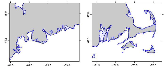
The diagram argues for a switch. A factor in such a decision, though, has to be storage requirements. The 1:10M file is 8.4 Mbyte as provided by Natural Earth, but it becomes a 3.0 Mbyte file in R format, which is to be compared with the 1.8 Mbyte file for the coastline that was used in Oce previously. The old coastline had 406694 points, while the 1:10m version has 552670 points (i.e. 30% more points); the mismatch between data-size ratio and file-size ratio perhaps has something to do with compression.
Part 2: global applications
As explained in Part 1, the existing coastline in oce is noticeably coarse on scales commonly used in coastal-ocean work. A better alternative is the 1:10m coastline provided at the Natural Earth website. That site also provides 1:50m and 1:100m versions, and this entry illustrates those as well, with an aim to deciding whether to include these in oce.
The files are named Existing (what is in oce as of early December 2013), Fine (the 1:10m file), Medium (the 1:50m file) and Coarse (the 1:100m file). The latter three were downladed 2013 Dec and read into Oce with names coastlineWorldFine etc, and then timing and graphical tests were done.
A world map was plotted to a PNG file (R file world.R, appendix 1), and it yielded the following times: Existing 6.3s, Fine 16.9s, Medium 0.63s, Coarse 0.14s. (For context, note that all four panels plot in under half a second with the x11 device commonly used for interactive work.) The corresponding size of the .rda files are: Existing 1.8Mb, Fine 3.0Mb, Medium 0.5Mb, and Coarse 0.1Mb.
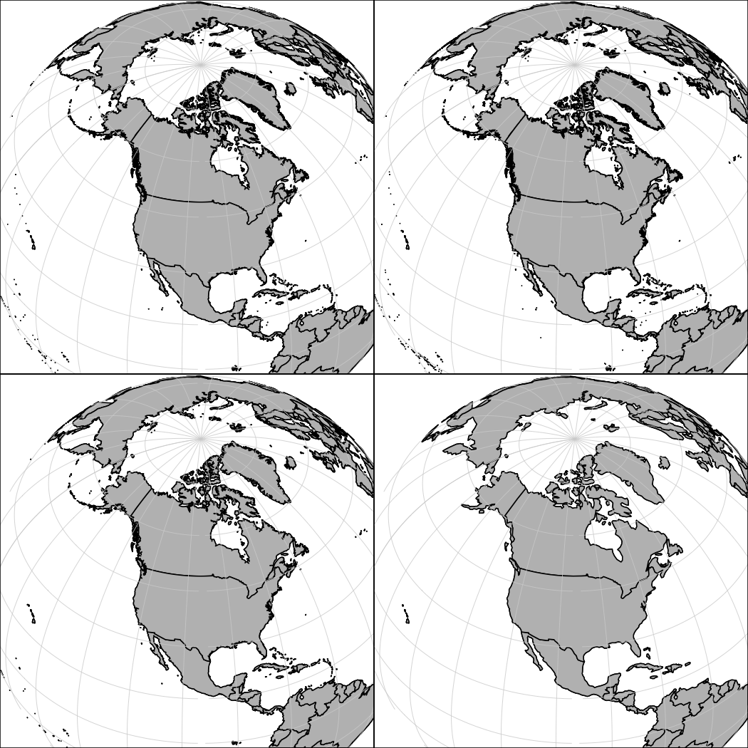
At top-left is the existing coastline, which on this scale is very close in appearance to the Fine resolution case to its right, and the Medium resolution case below it. At bottom right is the Coarse case, which produces very similar overall features but misses many islands (see e.g. near Alaska and the Caribbean). Timing tests reveal the Existing coastline file to take 6.3s, Fine 17s, Medium 0.63s, and Coarse 0.14s. This argues against the use of Fine for interactive work on even continental scales, with Medium seeming to be the best choice at global scales, with its order of magnitude reduction in plotting time. (As a side note, speed improvements will be reflected in file sizes if PDF output is chosen.) As for the shelf scale, see the previous posting, which suggests the use of Fine at such scales.
Discussion and conclusion
These results argue for replacing the existing coastline with the three variants from Natural Earth. This is also a good time to prune other datasets. Separate tests (not shown here) suggest that Fine is preferable to the present dataset named coastlineMaritimes, so the latter can be dropped. Oce also contains a dataset named coastlineSLE that is mainly of interest to the author (and, like any localized dataset, can always be loaded for detailed work).
Subject to feedback from other oce users, all three Natural Earth datasets will be incorporated into Oce. The existing coastline (named coastlineWorld) will be replaced with Medium. (Altering the name would break existing code.) The other datasets will be named coastlineFine and coastlineCoarse. The existing datasets for the Maritimes and SLE will be dropped. The changes will increase plot quality and speed, at the cost of a 1.7Mb increase in the size of the data package. The work will be done in a new branch called coastline that will hang off the branch called develop, and will be merged into the latter pending user approval and testing.
APPENDIX 1
The R code to make the first figure is provided below. Readers wishing to reproduce this will need to download the coastline file named in line 2, from the naturalearthdata website.
1
2
3
4
5
6
7
8
9
10
11
12
13
14
15
library(oce)
d <- read.oce("ne_10m_admin_0_countries.shp")

## Two panels illustrate two oceanographic centres.
par(mfrow=c(1,2))

## Left panel: Halifax NS, with grey for existing
## world coastline and blue for the 1:10m version
## under consideration.
plot(coastlineWorld, clon=-63.60, clat=44.65, span=200)
lines(d[['longitude']], d[['latitude']], col='blue', lwd=1.4)

## As left panel, but for Woods Hole MA.
plot(coastlineWorld, clon=-70.70, clat=41.65, span=200)
lines(d[['longitude']], d[['latitude']], col='blue', lwd=1.4)
APPENDIX 2
The R code used to make the second figure is given below. Readers should note that this will not work for them unless they first download the datasets, read the datasets with read.oce(), and save() the results in .rda files as named in the code.
1
2
3
4
5
6
7
8
9
10
11
12
13
14
15
16
17
18
19
20
21
22
23
24
25
library(oce)
load("coastlineWorldFine.rda")
load("coastlineWorldMedium.rda")
load("coastlineWorldCoarse.rda")
if (!interactive())
    png("world.png",width=7,height=7,unit='in',res=150,pointsize=7)
par(mfrow=c(2,2), mar=rep(0, 4))
system.time(mapPlot(coastlineWorld,
                    longitudelim=c(-80,10), latitudelim=c(0,120),
                    projection="orthographic", axes=FALSE,
                    orientation=c(45,-100,0), fill='grey'))
system.time(mapPlot(coastlineWorldFine,
                    longitudelim=c(-80,10), latitudelim=c(0,120),
                    projection="orthographic", axes=FALSE,
                    orientation=c(45,-100,0),fill='grey'))
system.time(mapPlot(coastlineWorldMedium,
                    longitudelim=c(-80,10), latitudelim=c(0,120),
                    projection="orthographic", axes=FALSE,
                    orientation=c(45,-100,0), fill='grey'))
system.time(mapPlot(coastlineWorldCoarse,
                    longitudelim=c(-80,10), latitudelim=c(0,120),
                    projection="orthographic", axes=FALSE,
                    orientation=c(45,-100,0), fill='grey'))
if (!interactive())
    dev.off()