Downloading and Plotting NOAA SST data
NOAA provides datasets of sea-surface temperature (SST) in NetCDF form, at
https://downloads.psl.noaa.gov/Datasets/noaa.oisst.v2.highres/. There are
many files to choose from, but for this exercise I’ll use the one named
sst.day.mean.2024.nc, which holds data for the year 2024. The example code shows how to do the work. The following notes may be of use.
- The data file holds a note referring to this dataset as “NOAA/NCEI 1/4 Degree Daily Optimum Interpolation Sea Surface Temperature (OISS T) Analysis, Version 2.1”; see the website for more information.
- The file is cached, to avoid the slow download.
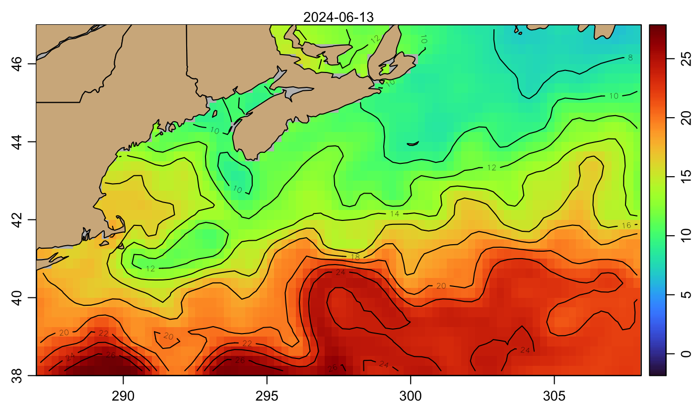
- This shows waters near Nova Scotia. Use the
looklonandlooklatvalues for other regions. - Adjusting the
widthparameter in thepng()call is a good way to remove white bands on either the left/right or top/bottom sides of the plot. - This plot shows the most recent dataset. Adjust the look to get other values. (Why a loop? Because my real goal is to make a movie…)
url <- "https://downloads.psl.noaa.gov/Datasets/noaa.oisst.v2.highres/"
file <- "sst.day.mean.2024.nc"
# Change cache to FALSE to force a download.  But note that it is a
# large file, so you're wise to experiment with plot aesthetics on
# a cached file.
cache <- TRUE
if (!cache || !file.exists(file)) { # takes about a minute
    download.file(paste0(url, file), file)
}
library(ncdf4)
library(oce)
data(coastlineWorldMedium, package = "ocedata")
# Cache variables to speed experimentation with plot aesthetics.
if (!exists("sstOrig")) {
    message("reading from ", file)
    nc <- nc_open(file)
    lonOrig <- ncvar_get(nc, "lon")
    latOrig <- ncvar_get(nc, "lat")
    sstOrig <- ncvar_get(nc, "sst")
    time <- ncvar_get(nc, "time")
    t <- as.POSIXct("1800-01-01 00:00:00", tz = "UTC") + time * 86400
    nc_close(nc)
}

looklon <- 287 <= lonOrig & lonOrig <= 308
looklat <- 38 <= latOrig & latOrig <= 47.0
lon <- lonOrig[looklon]
lat <- latOrig[looklat]
sst <- sstOrig[looklon, looklat, ]
sstdim <- dim(sst)
cm <- colormap(zlim = range(sst, na.rm = TRUE), col = oceColorsTurbo)
# Adjust height to avoid whitespace at top+bottom or left+right
if (!interactive()) {
    png("2024-06-15-sst.png",
        width = 7, height = 4.15, unit = "in", res = 200,
        pointsize = 10
    )
}
asp <- 1 / cospi(mean(range(lat)) / 180)
# Show most recent day
for (i in length(t)) {
    message(format(t[i]))
    imagep(lon, lat, sst[, , i],
        asp = asp, colormap = cm,
        mar = c(2.2, 2.2, 1.5, 0.5)
    )
    contour(lon, lat, sst[, , i],
        levels = seq(-2, 34, 2),
        drawlabels = !FALSE,
        add = TRUE
    )
    polygon(360 + coastlineWorldMedium[["longitude"]],
        coastlineWorldMedium[["latitude"]],
        col = "tan"
    )
    mtext(t[i])
}
dev.off()