Drawing Wind Barbs with the oce R Package

Introduction

Recently, an oce user named Max Dupilka asked (see https://github.com/dankelley/oce/issues/2191) whether oce could draw “wind-barb” diagrams. This struck me an oce co-author Clark Richards as a good idea. So, with a lot of help from Max, I added this feature.

After a few days of testing, the feature was inserted into the mapDirectionField() function (click that word to visit the help page).

In this blog entry, I’ll show how to use this function. First, though, you’ll need to see how to update your version of oce to the development version.

Gaining Access to the oce Update

This may not appear in

CRAN (https://cran.r-project.org/package=oce) for a few months, given CRAN policies on updates to packages. But, if you have a system that is set up to build R packages from source (which requires C, C++ and Fortran compilers), you can install the update by typing the following in an R session. (Install the remotes package first, if you don’t have it already.)

remotes::install_github("dankelley/oce", ref = "develop")

An Idealized Example

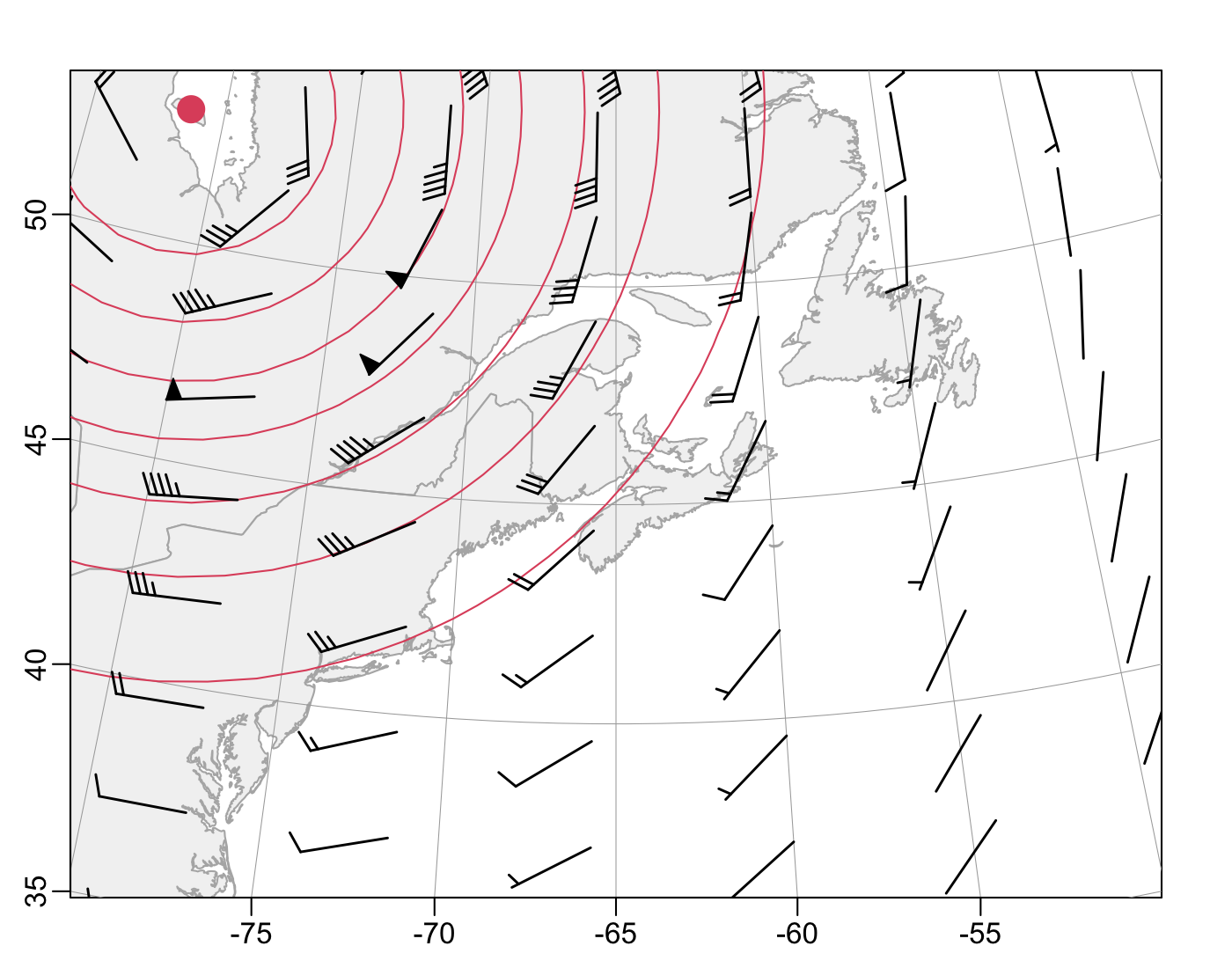
The diagram given above is an example. I created it by imagining Gaussian-shaped low-pressure zone centred over the southern part of Hudson’s Bay (visible as the red dot in the northwest region of the figure), and computing winds with the geostrophic formulae.

The code is at the bottom of this post. As you can see, I constructed a fairly dense grid of longitudes and latitudes to get smooth contours (red), but sub-sampled for the barbs. If I had not sub-sampled, the barbs would have been quite crowded. (You may also control the lengths of the wind indicators, and the widths of the barbs; type ?mapDirectionField to learn more.)

How to Read a Wind-Barb Diagram

If the speed at a given location is exactly zero, a dot is drawn there.

For non-zero speeds, a line segment is drawn in the upwind direction. The lengths of these segments are designed to cover equal distance over the ground (accounting for the projection used in the map).

If the speed is under 2.5 knots (i.e. if it rounds to 0), then the segment is all that is drawn. For higher speeds, barbs and pennants may be drawn, depending on the speed.

If the speed rounds to 5 knots, a single short barb is drawn near the end of the main segment. You can see one of these, extending from the southern edge of Newfoundland.

If the speed rounds to 10 knots, a long barb is drawn at the end.

For higher speeds, long and short barbs are drawn (the short ones closer to the origin point). For example, the long and short barb for winds near Cape Breton indicate a speed of 15 knots. This pattern continues until 50 knots is reached. At 50 knots a pennant (triangle) is drawn. You can see some pennants at towards the northeast of the diagram, where lines of constant pressure are closest together.

This scheme makes it easy to infer the speed at any spot. Start with 0 knots. Add 5 knots for each short barb. Then add 10 knots for each normal barb. And then add 50 knots for each pennant. The sum is the speed, rounded to 5 knots.

Using Other Units

I have seen displays use km/hour instead of knots, but retain the 5:10:50 scheme for short barbs, normal barbs, and pennants. Of course, it is easy to use mapDirectionField() to accommodate this or any other 5:10:50 scheme, simply by using a multiplier on velocity.

If your interest is in wind stress, consider using stress instead of velocity. For example, a rough value for wind speed over the North Atlantic is 10m/s. Using air density 1.2 kg/m^3 with a quadratic drag coefficient of 0.002 (say), this yields a stress of 0.24 Pa. This might suggest using short barbs could be used for stress increments of 0.1 Pa, normal barbs for 0.2 Pa, and pennants for 0.5 Pa.

R Code to Make the Example

library(oce)
data(coastlineWorldFine, package = "ocedata")
par(mar = rep(2, 4))
mapPlot(coastlineWorldFine,
    border = gray(0.7),
    col = grey(0.95),
    projection = "+proj=lcc +lat_1=40 +lat_2=60 +lon_0=-65",
    longitudelim = c(-80, -50), latitudelim = c(40, 50)
)
# fake a geostrophic wind field centred in lower Hudson's Bay
model <- function(x, y, latitude, R = 100e3, rho = 1.2,
                  highP = 101.5e3, lowP = 98e3) {
    E <- exp(-(x^2 + y^2) / R^2)
    deltaP <- highP - lowP
    P <- highP - deltaP * E
    dPdx <- 2 * deltaP * x / R^2 * E
    dPdy <- 2 * deltaP * y / R^2 * E
    f <- oce::coriolis(latitude)
    u <- -dPdy / rho / f
    v <- dPdx / rho / f
    list(P = P, dPdx = dPdx, dPdy = dPdy, u = u, v = v)
}

nlon <- 50
nlat <- nlon + 1
lon <- seq(-100, -30, length.out = nlon)
lat <- seq(30, 60, length.out = nlat)
g <- expand.grid(lon = lon, lat = lat)
xy <- lonlat2map(g$lon, g$lat)
xyc <- lonlat2map(-81.30, 53.01) # Akimiski Island (Hudson's Bay)
m <- model(xy$x - xyc$x, xy$y - xyc$y,
    latitude = g$lat, R = 1000e3, lowP = 97e3, highP = 101e3
)
mps2knot <- 1.94384 # 1 m/s is 1.94384 knots
u <- mps2knot * matrix(m$u, nrow = length(lon))
v <- mps2knot * matrix(m$v, nrow = length(lon))
P <- matrix(m$P, nrow = length(lon))
mapContour(lon, lat, P, drawlabels = FALSE, col = 2, lwd = 1)
lx <- seq(1, length(lon), 4)
ly <- seq(1, length(lat), 4)
mapDirectionField(lon[lx], lat[ly], u[lx, ly], v[lx, ly],
    lwd = 1.4,
    code = "barb", scale = 2, length = 0.25
)
points(xyc$x, xyc$y, pch = 20, cex = 3, col = 2)