Demonstration of the Updated mapImage Function in oce
I have been making some changes to the oce function mapImage() lately, to
address an issue kindly pointed out by a user on github^[1]. The problem is
that the image can have missing values at certain points, depending on the
projection being used, the geographical domain being shown, and the data grid
being plotted.
I won’t get into details here. I just want to illustrate the problem and some solutions. This requires the very latest version of the development branch of the oce code, as it will exist in perhaps a few days or weeks, once the issue is closed.
At the bottom of this post I have sample code. Notice that it has four
alternatives for the mapImage() call. The results from those alternatives
are pasted below.
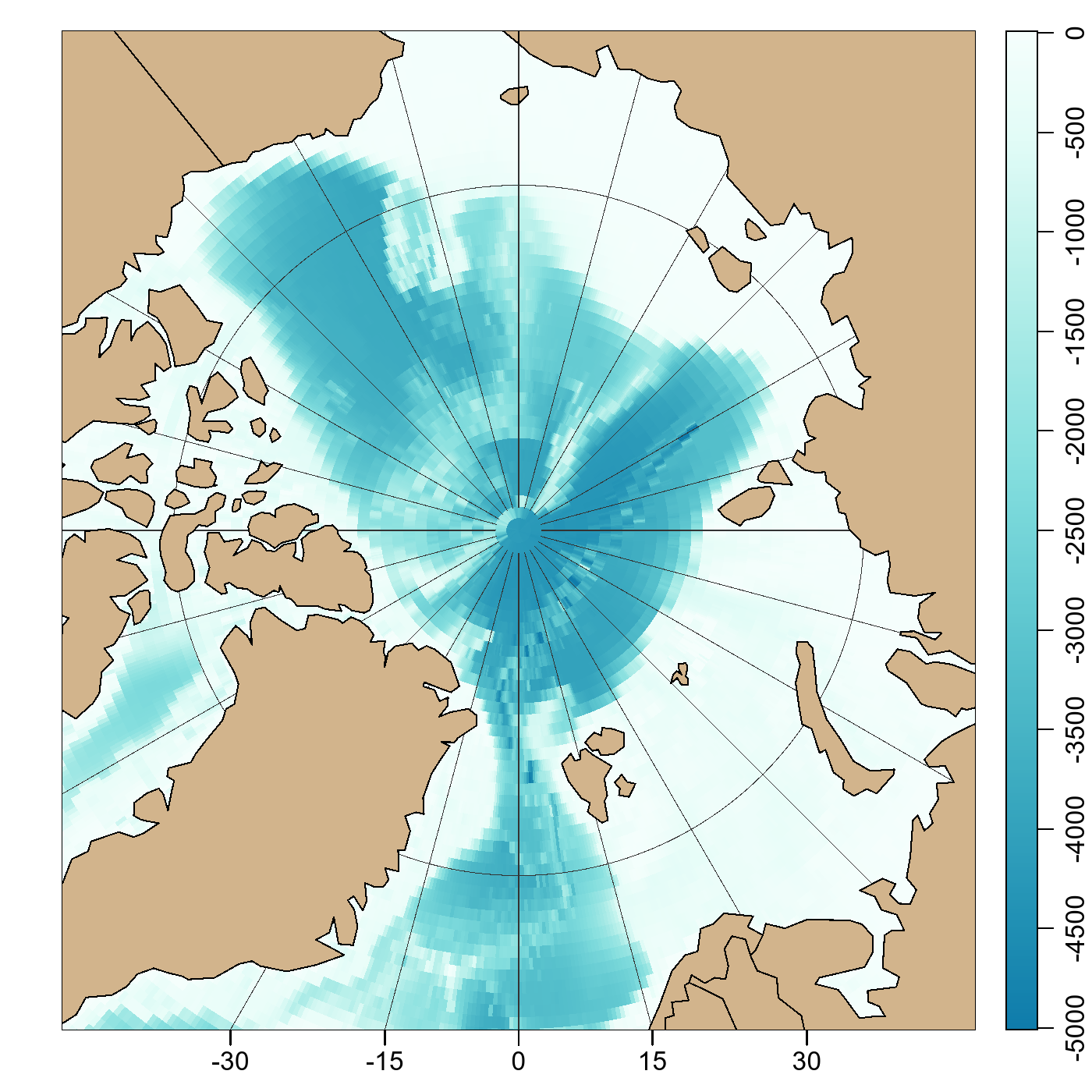
My preference is for option 1, which uses polygons for each longitude-latitude grid cell. It has the advantage, over the other methods, of showing the data faithfully.
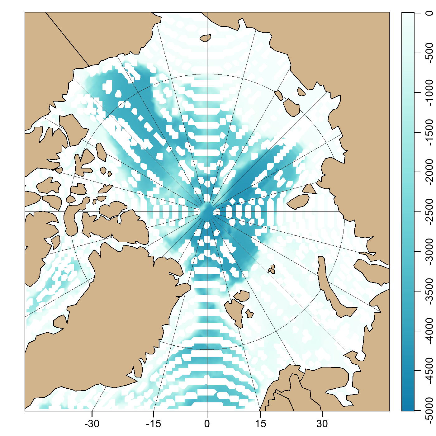
But sometimes filled contours are called for, perhaps because a smooth field is thought to be more appealing than a tiling of polygons. In this case, I would start with option 2. But if I see data gaps, as you can see below, I would move to either option 3 or option 4. There are pros and cons to both 3 and 4. Option 3 does some extra smoothing, which may be desired for noisy data. On the other hand, option 4 only alters the grid by filling in gaps, so it is closer to the original data.
The mapContour() function should also be considered. It has the advantage of
displaying contours without any of the gridding that is required for
mapContour() in options 2, 3 and 4. In other words, it is very close to the
data. However, contours for noisy fields can be very messy.
The bottom line is that the oce package offers a range of choices. The best choice depends on the nature of the data, as well as the intended audience.
Method 1: using polygons, not filled contours.
Method 2: using filled contours, yielding gaps.
Method 3: using filled contours, with larger grid cells to fill gaps.

Method 4: using filled contours, with a gridder that fills gaps.

Footnotes
Code
The images are made by uncommenting the various mapImage() blocks.
library(oce)
data(coastlineWorld)
data(topoWorld)

# Northern polar region, with color-coded bathymetry
par(mfrow = c(1, 1), mar = c(2, 2, 1, 1))
cm <- colormap(zlim = c(-5000, 0), col = oceColorsGebco)
drawPalette(colormap = cm)
mapPlot(coastlineWorld,
    projection = "+proj=stere +lat_0=90",
    longitudelim = c(-180, 180), latitudelim = c(70, 110)
)

# Method 1: the default, using polygons for lon-lat patches
mapImage(topoWorld, colormap = cm)

# Method 2: filled contours, with ugly missing-data traces
# mapImage(topoWorld, colormap = cm, filledContour = TRUE)

# Method 3: filled contours, with a double-sized grid cells
# mapImage(topoWorld, colormap = cm, filledContour = 2)

# Method 4: filled contours, with a gap-filling gridder)
# g <- function(...) binMean2D(..., fill = TRUE, fillgap = 2)
# mapImage(topoWorld, colormap = cm, filledContour = TRUE, gridder = g)


mapGrid(15, 15, polarCircle = 1, col = gray(0.2))
mapPolygon(coastlineWorld[["longitude"]],
    coastlineWorld[["latitude"]],
    col = "tan"
)