DE solution in R (nonlinear oscillator)
The function lsoda() from the deSolve package is a handy function for
solving differential equations in R. This is illustrated here with a classic
example: the nonlinear oscillator.
As explained in introductory Physics textbooks, the nonlinear oscillator equation dθ2/dt2 + sin θ = 0 can be simplified to a linear form d2θ/dt2 + θ = 0 provided that θ ≪ 1.
It is a simple matter to show that the linear form has solution θ = asin (t), given initial conditions θ = 0 and dθ/dt = a at time t=0.
Although the nonlinear form is harder to solve analytically, it is amenable to
numerical solution, using the lsoda() function provided by the deSolve
package.
The first step is to break the second-order DE down into two first-order DEs:
ϕ = dθ/dt and dϕ/dt = −sin θ. So, let’s give that a try. The method
used in lsoda() is for the user to create a function that has arguments for
time, t, solution initial conditions, y, and a list of mathematical
parameters called parms. With that information in hand, readers who
know R will likely be able to understand the following code.
library(deSolve)
de <- function(t, y, parms, ...)
{
    theta <- y[1]
    phi <- y[2]
    list(c(dthetadt=phi, dphidt=-sin(theta)))
}

a <- 0.1
y0 <- c(0, a)
t <- seq(0, 4*pi, pi/100)
sol <- lsoda(y=y0, times=t, func=de)
ylim <- max(range(sol[,2])) * c(-1, 1)
par(mar=c(3.5, 3.5, 1, 1), mgp=c(2, 0.7, 0))
plot(sol[,1], sol[,2], type='l', ylim=ylim, col='blue',
    xlab=expression(t), ylab=expression(theta(t)))
grid()
lines(t, a*sin(t), col='red', lty='dashed')
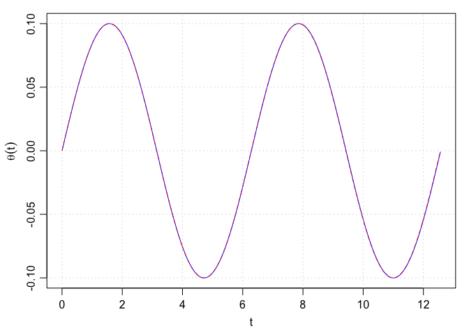
Notice that in this case, with a=0.1, the linear and nonlinear solutions coincide. What about higher values, though? To see, it might help to rewrite the code a bit, as follows
library(deSolve)
oscillator <- function(a=0.1)
{
    de <- function(t, y, parms, ...)
    {
        theta <- y[1]
        phi <- y[2]
        list(c(dthetadt=phi, dphidt=-sin(theta)))
    }
    y0 <- c(0, a)
    t <- seq(0, 8*pi, pi/100)
    sol <- lsoda(y=y0, times=t, func=de)
    ylim <- max(range(sol[,2])) * c(-1, 1)
    par(mar=c(3.5, 3.5, 1, 1), mgp=c(2, 0.7, 0))
    plot(sol[,1], sol[,2], type='l', ylim=ylim, col='blue',
         xlab=expression(t), ylab=expression(theta(t)))
    grid()
    lines(t, a*sin(t), col='red')
    legend("bottomleft", col=c("red", "blue"), lwd=1,
           legend=c("linear", "nonlinear"),
           bg="white")
}
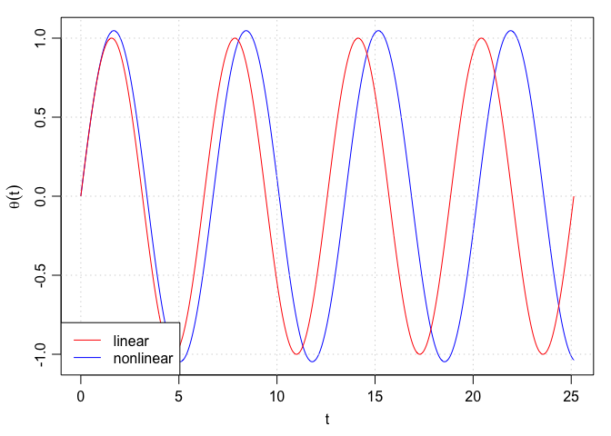
Here’s a somewhat nonlinear situation. Notice that the system still oscillates, albeit with high amplitude and longer period.
oscillator(1)
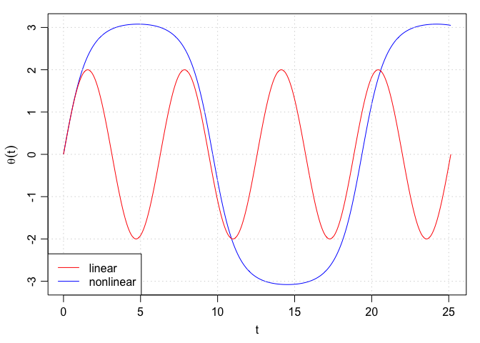
Now, let’s try a much more nonlinear situation, with a=1.999. As the following shows this system has quite a different character. Yes, it is still repeating, so it has not lost that behaviour. But the period has approximately doubled, and the peaks and valleys are now distinctly flatter than for a sinusoidal system.
oscillator(1.999)
What about for higher a values? I think I’ll leave that to readers. You have a simple experimental tool here, that you can use to explore the dynamics. The only parameter here is the value of a, so perhaps try some experiments with a range of a values, to see whether changes are slow across the board, or whether there might be some values of a at which large changes occur. Of course, you could search the web for answers to such questions, but where’s the fun in that, when you have a tool that will let you discover things for yourself?