Introduction

Box models are popular in some branches of oceanography and other geophysical disciplines, partly because they are simple to construct and to solve. This posting shows how to solve a box model in R, using the lsoda() function in the deSolve package.

The basic ideas can be explained in the context of riverine input into a lake that connects to the sea. Readers with mathematical expertise will see easily that the same method holds for a wide variety of problems. An oceanographer might think of salinity reduction. A meteorologist might think of the seasonal lag of ocean temperature. A pharmacologist might think of the concentration of a drug in the bloodstream. A contractor might think of water in a basement. But let’s stick to the lake, shall we?

Model formulation

Let the lake surface area be A, and its water level be h, with the latter being expressed as height above (constant) sea level. Let the river input volume per unit time be R. Suppose that the lake drains into the sea with volume output per unit time given by a linear law (as perhaps with pressure-driven viscous flow) of the form \(\gamma h\) where the coefficient has units of area per time.

The principle of volume conservation yields the differential equation

\[A\frac{dh}{dt} = R - \gamma h\]

Here, the left-hand side is the changing volume of the lake (assuming vertical coastline). In this equation, R (with units m\(^3\)/s) may vary with time as rivers flow and ebb, driven by rainfall or perhaps spring snow-melt.

In many circumstances it would make sense to non-dimensionalize the equation at this point, but for practical purposes it can be convenient to retain physical units. For example, the task could be to find the response to an observed time series \(R=R(t)\) of forcing.

Expressing the model as

\[\frac{dh}{dt} = \frac{R-\gamma h}{A}\]

is helpful since this is a form that works well with lsoda(), the R function to be used here to carry out the numerical integration of the differential equation.

Solution in R

The first step is to load the package containing lsoda().

library(deSolve)

Readers who are following along might want to type ?lsoda in an R console at this point, to get an idea of the reasoning being followed here. The summary is that lsoda() takes initial conditions as its first argument, a vector of times at which to report the solution as its second argument, a function defining the differential equation(s) as its third argument, and a list containing model parameters in its fourth argument.

We start by defining initial conditions, in line 1. In this case, suppose that h=0, i.e. that the lake water level is equal to that of the sea. Then, in line 2, we set parameters. This is at the heart of the matter, and will be the most important part of any application of such a model. Here, we take simple values: \(h=0\) initially, a lake of area \(A=4\times 10^6\) m\(^2\), and outflow coefficient \(\gamma=20\) m\(^2\)/s.

IC <- 0
parms <- list(A = 4e6, gamma = 20)

Suppose we would like to examine the result of riverine input \(R\) varying from a base value of 1 m\(^3\)/s to a one-day increase to 10 m\(^3\)/s. We may do that as follows. Note that the steady-state solution for the lower value of \(R\) is shown with a dotted line.

sperday <- 86400 # seconds per day
times <- seq(0, 20*sperday, length.out = 500)
R <- function(t)
{
    1 + ifelse(10 * sperday < t & t < 11 * sperday, 9, 0)
}

(The length of times mainly matters to plotting; it has no effect on the accuracy of the solution, i.e. we are not setting an integration time step here.)

Next, set up the differential equation. This has to follow a certain format. The function must take time as first argument, current model state (a vector, generally) as second, and parameters, third. The function returns a list of derivatives.

DE <- function(t, y, parms)
{
    h <- y[1]
    dhdt <- (R(t) - parms$gamma * h) / parms$A
    list(dhdt)
}

Here, the state is extracted into a variable named h and the derivative is stored in a variable named dhdt. This is done merely for clarity of illustration here; experienced programmers are likely to write DE as a single-line function.

Computing the model solution is now easy:

sol <- lsoda(IC, times, DE, parms)

defines sol, which has time as its first column and the solution as its second. We may plot the results as follows (where time is indicated in days for simplicity).

Results

par(mfrow=c(2,1), mar=c(3,3,1,1), mgp=c(2,0.7,0))
h <- sol[,2]
Day <- times / 86400
plot(Day, R(times), type='l', ylab="River input [m^3/s]")
plot(Day, h, type='l', ylab="Lake level [m]")
abline(h = 1 / parms$gamma, lty = 2) # theoretical steady state for 1 m^3/s

Box-model results.

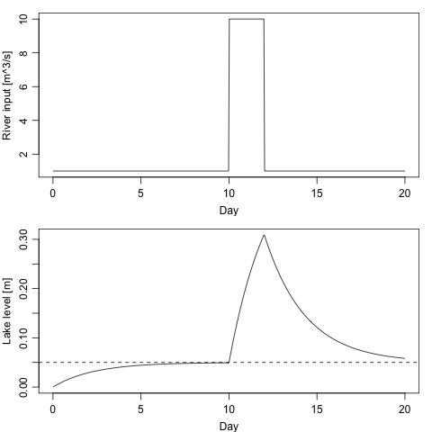
In this case, the model is so simple that there is no real need for a numerical simulation, but this would not be true if, say, realistically-varying \(R(t)\) forcing was applied, if \(\gamma\) were parameterized to vary with \(h\) or \(dh/dt\), etc.

Conclusions

Those interested in box models might like to alter the parameters and forcing function, to study the results.

Adding more boxes is easy, and a good exercise for the reader. Careful adjustment of parameters in multi-box models can yield reasonably useful alternatives to high-resolution numerical models, especially for exploratory work.

It is also a simple matter to change the forcing and the model formulation. For example, the outflow function could be made nonlinear, e.g. to account for hydraulic-control effects. Adding time dependence to parameterizations is not difficult either, and it opens the possibility of using such models in wide applications, e.g. modelling dam-break situations.

At a more advanced level, one can also use such a model in a data-assimilative way to infer parameter values from observations of quantities predicted by the model. For example, if lake area and river input were known for a given lake then observations of lake level (compared with sea level) could yield a value of \(\gamma\) as formulated here, or formulated in a more sophisticated way, e.g. depending on \(dh/dt\), etc.

As mathematically-inclined readers might agree, and others might learn by a bit of exploration, numerical experimentation can be a useful tool for increasing understanding.