PISA scores

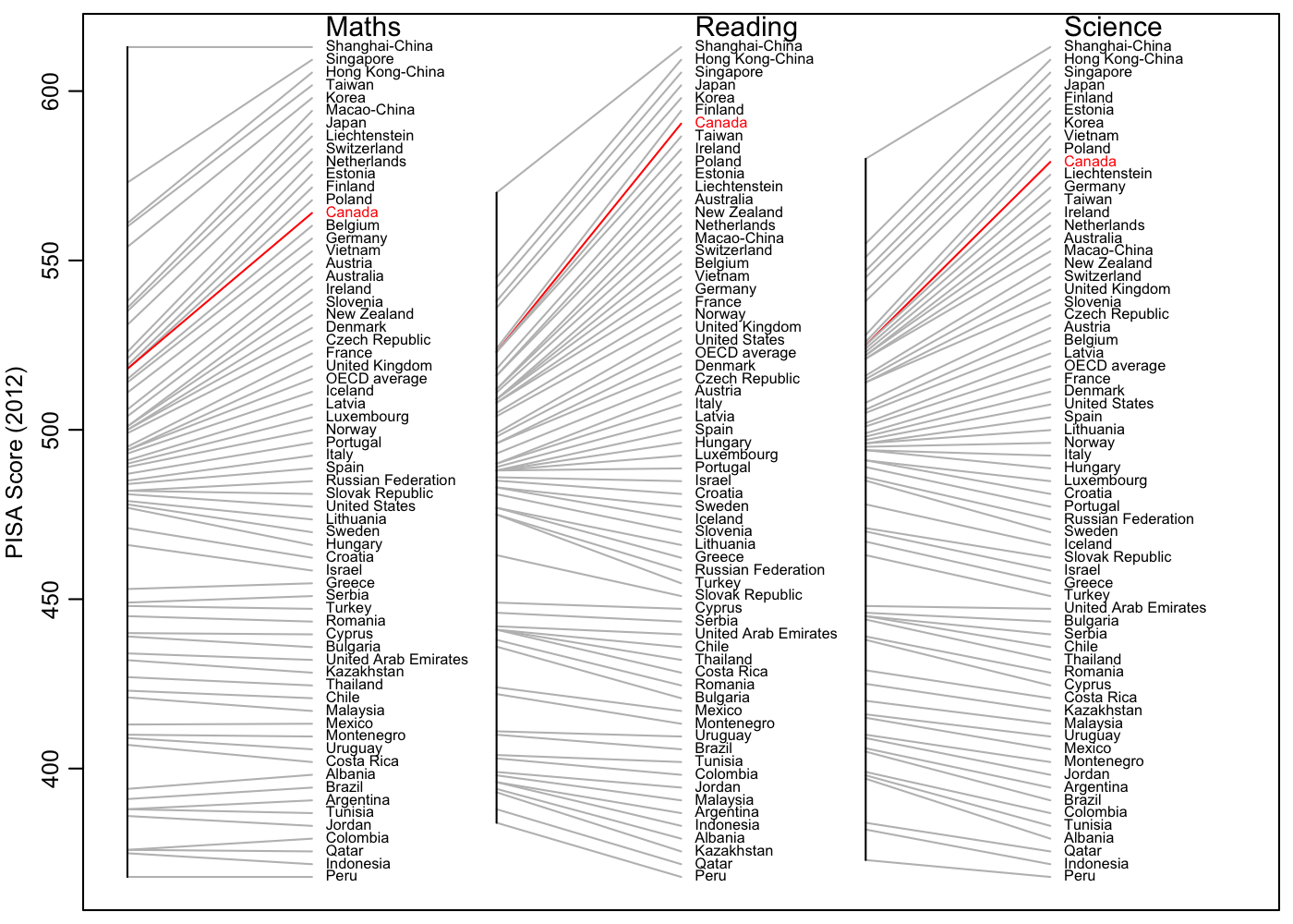
The Guardian Newspaper had an interesting article about the Pisa (Program for International Student Assessment) scores for 2012, and it included data. Since I was interested to see how my own region scored, I downloaded the data into a file called PISA-summary-2012.csv and created a plot summarizing scores in all the sampled regions, with Canada highlighted.

I think the graphs speak for themselves.

Code

png("2014-01-06-pisa-scores.png",
    unit = "in", width = 7, height = 5,
    res = 200, pointsize = 9
)
# Define data (avoids attaching a file to this blog entry)
data <- "
1,Shanghai-China,613,3.8,55.4,4.2,570,4.6,580,1.8
3,Hong Kong-China,561,8.5,33.7,1.3,545,2.3,555,2.1
2,Singapore,573,8.3,40,3.8,542,5.4,551,3.3
7,Japan,536,11.1,23.7,0.4,538,1.5,547,2.6
12,Finland,519,12.3,15.3,-2.8,524,-1.7,545,-3
11,Estonia,521,10.5,14.6,0.9,516,2.4,541,1.5
5,Korea,554,9.1,30.9,1.1,536,0.9,538,2.6
17,Vietnam,511,14.2,13.3,m,508,m,528,m
14,Poland,518,14.4,16.7,2.6,518,2.8,526,4.6
13,Canada,518,13.8,16.4,-1.4,523,-0.9,525,-1.5
8,Liechtenstein,535,14.1,24.8,0.3,516,1.3,525,0.4
16,Germany,514,17.7,17.5,1.4,508,1.8,524,1.4
4,Taiwan,560,12.8,37.2,1.7,523,4.5,523,-1.5
20,Ireland,501,16.9,10.7,-0.6,523,-0.9,522,2.3
10,Netherlands,523,14.8,19.3,-1.6,511,-0.1,522,-0.5
19,Australia,504,19.7,14.8,-2.2,512,-1.4,521,-0.9
6,Macao-China,538,10.8,24.3,1,509,0.8,521,1.6
23,New Zealand,500,22.6,15,-2.5,512,-1.1,516,-2.5
9,Switzerland,531,12.4,21.4,0.6,509,1,515,0.6
26,United Kingdom,494,21.8,11.8,-0.3,499,0.7,514,-0.1
21,Slovenia,501,20.1,13.7,-0.6,481,-2.2,514,-0.8
24,Czech Republic,499,21,12.9,-2.5,493,,508,-1
18,Austria,506,18.7,14.3,0,490,-0.2,506,-0.8
15,Belgium,515,18.9,19.4,-1.6,509,0.1,505,-0.8
28,Latvia,491,19.9,8,0.5,489,1.9,502,2
-,OECD average,494,23.1,12.6,-0.3,496,0.3,501,0.5
25,France,495,22.4,12.9,-1.5,505,0,499,0.6
22,Denmark,500,16.8,10,-1.8,496,0.1,498,0.4
36,United States,481,25.8,8.8,0.3,498,-0.3,497,1.4
33,Spain,484,23.6,8,0.1,488,-0.3,496,1.3
37,Lithuania,479,26,8.1,-1.4,477,1.1,496,1.3
30,Norway,489,22.3,9.4,-0.3,504,0.1,495,1.3
32,Italy,485,24.7,9.9,2.7,490,0.5,494,3
39,Hungary,477,28.1,9.3,-1.3,488,1,494,-1.6
29,Luxembourg,490,24.3,11.2,-0.3,488,0.7,491,0.9
40,Croatia,471,29.9,7,0.6,485,1.2,491,-0.3
31,Portugal,487,24.9,10.6,2.8,488,1.6,489,2.5
34,Russian Federation,482,24,7.8,1.1,475,1.1,486,1
38,Sweden,478,27.1,8,-3.3,483,-2.8,485,-3.1
27,Iceland,493,21.5,11.2,-2.2,483,-1.3,478,-2
35,Slovak Republic,482,27.5,11,-1.4,463,-0.1,471,-2.7
41,Israel,466,33.5,9.4,4.2,486,3.7,470,2.8
42,Greece,453,35.7,3.9,1.1,477,0.5,467,-1.1
44,Turkey,448,42,5.9,3.2,475,4.1,463,6.4
48,United Arab Emirates,434,46.3,3.5,m,442,m,448,m
47,Bulgaria,439,43.8,4.1,4.2,436,0.4,446,2
43,Serbia,449,38.9,4.6,2.2,446,7.6,445,1.5
51,Chile,423,51.5,1.6,1.9,441,3.1,445,1.1
50,Thailand,427,49.7,2.6,1,441,1.1,444,3.9
45,Romania,445,40.8,3.2,4.9,438,1.1,439,3.4
46,Cyprus,440,42,3.7,m,449,m,438,m
56,Costa Rica,407,59.9,0.6,-1.2,441,-1,429,-0.6
49,Kazakhstan,432,45.2,0.9,9,393,0.8,425,8.1
52,Malaysia,421,51.8,1.3,8.1,398,-7.8,420,-1.4
55,Uruguay,409,55.8,1.4,-1.4,411,-1.8,416,-2.1
53,Mexico,413,54.7,0.6,3.1,424,1.1,415,0.9
54,Montenegro,410,56.6,1,1.7,422,5,410,-0.3
61,Jordan,386,68.6,0.6,0.2,399,-0.3,409,-2.1
59,Argentina,388,66.5,0.3,1.2,396,-1.6,406,2.4
58,Brazil,391,67.1,0.8,4.1,410,1.2,405,2.3
62,Colombia,376,73.8,0.3,1.1,403,3,399,1.8
60,Tunisia,388,67.7,0.8,3.1,404,3.8,398,2.2
57,Albania,394,60.7,0.8,5.6,394,4.1,397,2.2
63,Qatar,376,69.6,2,9.2,388,12,384,5.4
64,Indonesia,375,75.7,0.3,0.7,396,2.3,382,-1.9
65,Peru,368,74.6,0.6,1,384,5.2,373,1.3"

# Read the data and set up axes.
regionHighlight <- "Canada"
d <- read.csv(
    text = data, header = FALSE,
    col.names = c(
        "rank", "region",
        "math", "mathLow", "mathHigh", "mathChange",
        "reading", "readingChange",
        "science", "scienceChange"
    )
)
n <- length(d$math)
par(mar = c(0.5, 3, 0.5, 0.5), mgp = c(2, 0.7, 0))
range <- range(c(d$math, d$reading, d$science))
plot(c(0, 6), range,
    type = "n", xlab = "", axes = FALSE,
    ylab = "PISA Score (2012)"
)
axis(2)
box()
# Set parameters for label placement.
dy <- diff(par("usr")[3:4]) / 50
x0 <- 0
dx <- 1
cex <- 0.65

# Math scores
o <- order(d$math, decreasing = TRUE)
y <- approx(1:n, seq(range[2], range[1], length.out = n), 1:n)$y
segments(rep(x0, n), d$math[o], rep(x0 + dx, n), y,
    col = ifelse(d$region[o] == regionHighlight, "red", "gray")
)
lines(rep(x0, 2), range(d$math))
text(rep(x0 + dx, n), y, d$region[o],
    pos = 4, cex = cex,
    col = ifelse(d$region[o] == regionHighlight, "red", "black")
)
text(x0 + dx, range[2] + dy, "Maths", pos = 4, cex = 1.2)

# Reading scores
x0 <- x0 + 2 * dx
o <- order(d$reading, decreasing = TRUE)
segments(rep(x0, n), d$reading[o], rep(x0 + dx, n), y,
    col = ifelse(d$region[o] == regionHighlight, "red", "gray")
)
lines(rep(x0, 2), range(d$reading))
text(rep(x0 + dx, n), y, d$region[o],
    pos = 4, cex = cex,
    col = ifelse(d$region[o] == regionHighlight, "red", "black")
)
text(x0 + dx, range[2] + dy, "Reading", pos = 4, cex = 1.2)

# Science scores.
x0 <- x0 + 2 * dx
o <- order(d$science, decreasing = TRUE)
segments(rep(x0, n), d$science[o], rep(x0 + dx, n), y,
    col = ifelse(d$region[o] == regionHighlight, "red", "gray")
)
lines(rep(x0, 2), range(d$science))
text(rep(x0 + dx, n), y, d$region[o],
    pos = 4, cex = cex,
    col = ifelse(d$region[o] == regionHighlight, "red", "black")
)
text(x0 + dx, range[2] + dy, "Science", pos = 4, cex = 1.2)