Introduction

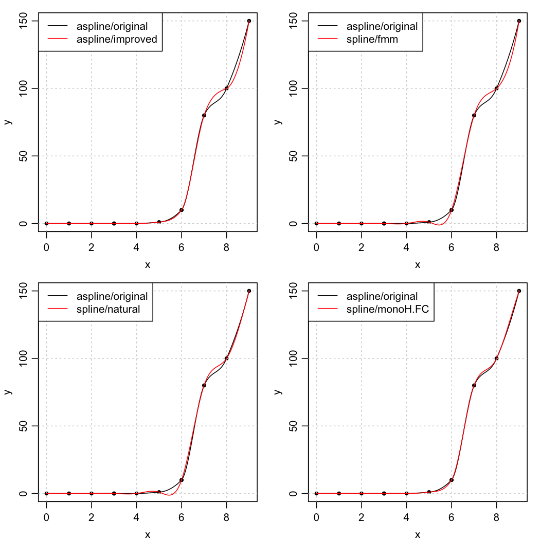
This follows up on the previous posting, using data provided by Akima (1972). The four panels of the plot produced by the following code compare the original Akima spline formula with an improved version, and three styles of spline() fits.

As noted in the code, two spline() methods are useless for general tasks and are ignored here. The "period" method sets the endpoint y-values equal, which will be useless in most applications. The "hyman" method requires the y values to be increasing, which again is useless in most applications.

Methods

The code first creates the data, the MD=1 case of Akima (1972), and defines xx as a finer-resolution version of x for plotting. Then it defines a function start for common operations on each panel, and then it displays comparisons. The idea of showing each in reference to the original akima method is to guide the eye, since plotting all in one panel makes a tangle that is difficult to grasp.

1
2
3
4
5
6
7
8
9
10
11
12
13
14
15
16
17
18
19
20
21
22
23
24
25
26
27
28
29
30
31
32
33
34
35
36
37
38
39
40
41
42
43
44
45
if (!interactive()) png("splines2.png", width=7, height=7, unit="in", res=150, pointsize=8)

## Data from "MD=1" set of akima1972iasc
x <- c(0, 1, 2, 3, 3, 4, 5,  6,  6,  7,   8,   9)
y <- c(0, 0, 0, 0, 0, 0, 1, 10, 10, 80, 100, 150)

## A mesh for plotting
xx <- seq(min(x), max(x), length.out=200)

library(akima)                         # for aspline()

start <- function()
{
    plot(x, y, pch=20)
    grid()
    akima <- aspline(x, y, xx, method="original")
    lines(akima$x, akima$y, lty=1)
}

par(mar=c(3, 3, 1, 1), mgp=c(2, 0.7, 0), mfrow=c(2,2))

start()
akima <- aspline(x, y, xx, method="improved")
lines(akima$x, akima$y, col=2)
legend("topleft", lwd=1, col=1:2, legend=c("aspline/original", "aspline/improved"), bg="white")

start()
fun <- splinefun(x, y, method="fmm")
lines(xx, fun(xx), col=2)
legend("topleft", lwd=1, col=1:2, legend=c("aspline/original", "spline/fmm"), bg="white")


start()
fun <- splinefun(x, y, method="natural")
lines(xx, fun(xx), col=2)
legend("topleft", lwd=1, col=1:2, legend=c("aspline/original", "spline/natural"), bg="white")


start()
fun <- splinefun(x, y, method="monoH.FC")
lines(xx, fun(xx), col=2)
legend("topleft", lwd=1, col=1:2, legend=c("aspline/original", "spline/monoH.FC"), bg="white")


if (!interactive()) dev.off()

Results

Conclusions

1. spline() with method="natural" or "fmm" produces undesirable wiggles (for x between 5 and 6).

2. spline() with method="monoH.FC" produces results that re very similar to aspline() with method="original".

3. Arguably, aspline() with method="original" produces results most similar to what one might draw by hand; as just noted, spline() with method="monoH.FC" produces essentially equivalent results.

4. It would be a bad idea to base general selection on just this one test, but the code provided here is easy to modify for real data (alter lines 5 and 6), so this posting may be useful to readers.

Citations

Hiroshi Akima, 1972. Algorithm 433 Interpolation and smooth curve fitting based on local procedures (E2). Communications of the Association for Computing Machinery, 15(10): 914-918.